Theano for solving Partial Differential Equation problems

We all know Theano as a forefront library for Deep Learning research. However, it should be noted that Theano is a general purpose numerical computing library, like Numpy. Hence, in this post, we will look at the implementation of PDE simulation in Theano.

The Laplace Equation

We will look at a simple PDE example, the Laplace Equation:

In other words, this is an second order PDE, as, recall that Laplacian in calculus is the divergence of gradient of a function:

particularly, in two dimension:

This simple equation could be solved by using Finite Difference scheme [1].

Note that in this example, we are ignoring the boundary value problem.

Solving Laplace Equation in Numpy

The Finite Difference solution of Laplace Equation is to repeatedly averaging the neighbors of a particular point:

This iterative solution is very simple to implement in Numpy. But first, let’s give this problem an initial condition:

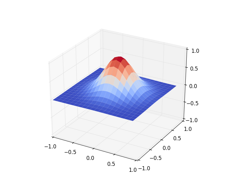
Visualizing the function:

Now, let’s implement this. First, we create the mesh, the solution space:

# Create 21x21 mesh grid
m = 21
mesh_range = np.arange(-1, 1, 2/(m-1))
x, y = np.meshgrid(mesh_range, mesh_range)

# Initial condition
U = np.exp(-5 \* (x**2 + y**2))

We then create an indexing scheme that select the point north, west, south, and east of any given point. We do this so that we could implement this in vectorized manner.

# [1, 2, ... , 19, 19]
n = list(range(1, m-1)) + [m-2]
e = n

# [0, 0, 1, 2, ... , 18]
s = [0] + list(range(0, m-2))
w = s

Having those indices, we could translate the PDE solution above in the code:

def pde_step(U):
    return (U[n, :]+U[:, e]+U[s, :]+U[:, w])/4.

Finally, we iteratively apply this update function.

U_step = U

for it in range(500):
    U_step = pde_step(U_step)

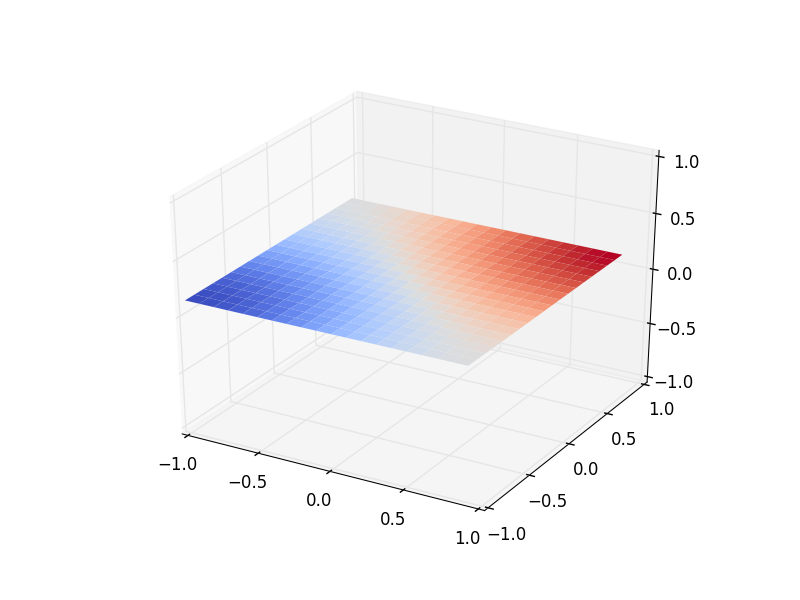
Here is the result:

Again, as we do not consider boundary value problem, the surface is diminishing until it is flat.

From Numpy to Theano

Translating the Numpy code to Theano is straightforward with caveat. The only thing different in the initialization is the variables: instead of Numpy array, we are now using Theano tensor.

import theano as th
from theano import tensor as T

# Create 21x21 mesh grid

m = 21
mesh_range = np.arange(-1, 1, 2/(m-1))
x_arr, y_arr = np.meshgrid(mesh_range, mesh_range)

# Initialize variables

x, y = th.shared(x_arr), th.shared(y_arr)
U = T.exp(-5 \* (x**2 + y**2))

n = list(range(1, m-1)) + [m-2]
e = n
s = [0] + list(range(0, m-2))
w = s

def pde_step(U):
return (U[n, :]+U[:, e]+U[s, :]+U[:, w])/4.

We are using Theano’s shared variables for our mesh variables as they are constants.

In the iteration part, things get little more interesting. In Theano, we replace loop with scan function. It is unintuitive at first, though.

k = 5

# Batch process the PDE calculation, calculate together k steps

result, updates = th.scan(fn=pde_step, outputs_info=U, n_steps=k)
final_result = result[-1]
calc_pde = th.function(inputs=[U], outputs=final_result, updates=updates)

What it does is to apply function pde_step repeatedly for k steps, and we initialize the tensor we are interested in with the initial state of U.

The output of this scan function is the result of each time step, in this case, there are k results. Hence, as we are only interested in the latest state of U (or \( \phi \)), we just pluck the last result.

Finally, we wrap this into a Theano’s function. The input is the current value of U and the output is U after applying pde_step, k times on U.

U_step = U.eval()

for it in range(100): # Every k steps, draw the graphics
    U_step = calc_pde(U_step)
    draw_plot(x_arr, y_arr, U_step)

We could think of our calc_pde as a batch processing of k iterations of our PDE. After each batch, we could use the latest U for e.g. visualization.

We might ask ourselves, do we need k to be greater than one? Definitely yes, as at every function call, we are sending our matrices from CPU to GPU, and receive them back. Low value of k definitely introduces overhead.

Why not TensorFlow?

TensorFlow is definitely an interesting library, on par with Theano in Deep Learning domain. However, the problem with TensorFlow is that it is still not very mature.

This piece of codes:

n = list(range(1, m-1)) + [m-2]
e = n
s = [0] + list(range(0, m-2))
w = s

def pde_step(U):
    return (U[n, :]+U[:, e]+U[s, :]+U[:, w])/4.

does not have any difference at all in Numpy and Theano version. However, we could not do this (at least easily) in TensorFlow.

Feature and behavior parity with Numpy is definitely a big factor, and it seems Theano is in front of TensorFlow in this regard, at least for now.

References

In this post we looked at a very simple Finite Difference solution of Laplace Equation. We implemented it in both Numpy and Theano.

Although Theano could be non-intuitive, especially in loop, it has better parity to Numpy compared to TensorFlow.

The full code, both in Numpy and Theano, could be found here: https://gist.github.com/wiseodd/c08d5a2b02b1957a16f886ab7044032d.

References

Mitra, Ambar K. “Finite difference method for the solution of Laplace equation.” preprint.