September 2015, at the ImageNet Large Scale Visual Recognition Challenge’s (ILSVRC) winners announcement, there was this one net by MSRA that dominated it all: Residual Net (ResNet) (He et al., 2015). The ensemble of ResNets crushing the classification task of other competitiors and almost halving the error rate of the 2014 winner.
Aside from winning the ILSVRC 2015 classification, ResNet also won the detection and localization challenge of the said competition. Additionally, it also won the MSCOCO detection and segmentation challenge. Quite a feat!
So, what makes ResNet so good? What’s the difference compared to the previous convnet models?
ResNet: the intuition behind it
The authors of ResNet observed, no matter how deep a network is, it should not be any worse than the shallower network. That’s because if we argue that neural net could approximate any complicated function, then it could also learn identity function, i.e. input = output, effectively skipping the learning progress on some layers. But, in real world, this is not the case because of the vanishing gradient and curse of dimensionality problems.

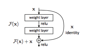
Hence, it might be useful to explicitly force the network to learn an identity mapping, by learning the residual of input and output of some layers (or subnetworks). Suppose the input of the subnetwork is
So that’s the difference between ResNet and traditional neural nets. Where traditional neural nets will learn
During backpropagation, learning residual gives us nice property. Because of the formulation, the network could choose to ignore the gradient of some subnetworks, and just forward the gradient from higher layers to lower layers without any modification. As an extreme example, this means that ResNet could just forward gradient from the last layer, e.g. layer 151, directly to the first layer. This gives ResNet additional nice to have option which might be useful, rather than just strictly doing computation in all layers.
ResNet: implementation detail
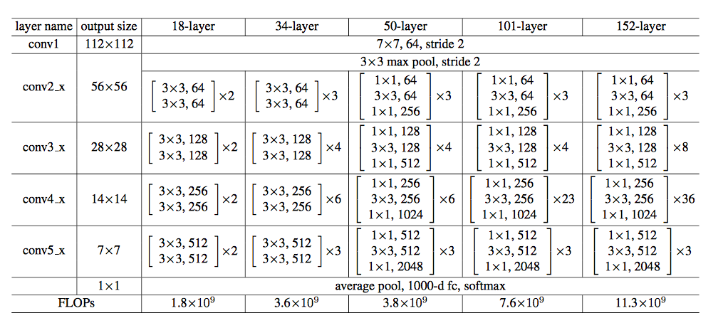
He et al. experimented with 152 layers deep ResNet in their paper. But due to our (my) monitor budget, we will look at the 34 layers version instead. Furthermore, it’s easier to understand with not so many layers, isn’t it?

At the first layer, ResNet use 7x7 convolution with stride 2 to downsample the input by the order of 2, similar to pooling layer. Then it’s followed by three identity blocks before downsampling again by 2. The downsampling layer is also a convolution layer, but without the identity connection. It continues like that for several layer deep. The last layer is average pooling which creates 1000 feature maps (for ImageNet data), and average it for each feature map. The result would be 1000 dimensional vector which then fed into Softmax layer directly, so it’s fully convolutional.
In the paper, He et al. use bottleneck architecture for each the residual block. It means that the residual block consists of 3 layers in this order: 1x1 convolution - 3x3 convolution - 1x1 convolution. The first and the last convolution is the bottleneck. It mostly just for practical consideration, as the first 1x1 convolution is being used to reduce the dimensionality, and the last 1x1 convolution is to restore it. So, the same network is now become 50 layers.

Notice, in 50 layers and more ResNet, at each block, there are now two 1x1 convolution layers.
References
- He, Kaiming, et al. “Deep residual learning for image recognition.” arXiv preprint arXiv:1512.03385 (2015).
- Szegedy, Christian, Sergey Ioffe, and Vincent Vanhoucke. “Inception-v4, inception-resnet and the impact of residual connections on learning.” arXiv preprint arXiv:1602.07261 (2016).
- Huang, Gao, Zhuang Liu, and Kilian Q. Weinberger. “Densely Connected Convolutional Networks.” arXiv preprint arXiv:1608.06993 (2016).