Natural Gradient Descent

Previously, we looked at the Fisher Information Matrix. We saw that it is equal to the negative expected Hessian of log likelihood. Thus, the immediate application of Fisher Information Matrix is as drop-in replacement of Hessian in second order optimization algorithm. In this article, we will look deeper at the intuition on what excatly is the Fisher Information Matrix represents and what is the interpretation of it.

Distribution Space

As per previous article, we have a probabilistic model represented by its likelihood . We want to maximize this likelihood function to find the most likely parameter . Equivalent formulation would be to minimize the loss function , which is the negative log likelihood.

Usual way to solve this optimization is to use gradient descent. In this case, we are taking step which direction is given by . This is the steepest descent direction around the local neighbourhood of the current value of in the parameter space. Formally, we have

The above expression is saying that the steepest descent direction in parameter space is to pick a vector , such that the new parameter is within the -neighbourhood of the current parameter , and we pick that minimize the loss. Notice the way we express this neighbourhood is by the means of Euclidean norm. Thus, the optimization in gradient descent is dependent to the Euclidean geometry of the parameter space.

Meanwhile, if our objective is to minimize the loss function (maximizing the likelihood), then it is natural that we taking step in the space of all possible likelihood, realizable by parameter . As the likelihood function itself is a probability distribution, we call this space distribution space. Thus it makes sense to take the steepest descent direction in this distribution space instead of parameter space.

Which metric/distance then do we need to use in this space? A popular choice would be KL-divergence. KL-divergence measure the “closeness” of two distributions. Although as KL-divergence is non-symmetric and thus not a true metric, we can use it anyway. This is because as goes to zero, KL-divergence is asymptotically symmetric. So, within a local neighbourhood, KL-divergence is approximately symmetric [1].

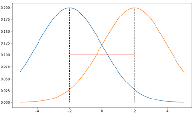
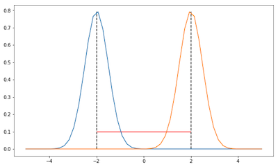
We can see the problem when using only Euclidean metric in parameter space from the illustrations below. Consider a Gaussian parameterized by only its mean and keep the variance fixed to 2 and 0.5 for the first and second image respectively:

In both images, the distance of those Gaussians are the same, i.e. 4, according to Euclidean metric (red line). However, clearly in distribution space, i.e. when we are taking into account the shape of the Gaussians, the distance is different in the first and second image. In the first image, the KL-divergence should be lower as there is more overlap between those Gaussians. Therefore, if we only work in parameter space, we cannot take into account this information about the distribution realized by the parameter.

Fisher Information and KL-divergence

One question still needs to be answered is what exactly is the connection between Fisher Information Matrix and KL-divergence? It turns out, Fisher Information Matrix defines the local curvature in distribution space for which KL-divergence is the metric.

Claim: Fisher Information Matrix is the Hessian of KL-divergence between two distributions and , with respect to , evaluated at .

Proof.    KL-divergence can be decomposed into entropy and cross-entropy term, i.e.:

The first derivative wrt. is:

The second derivative is:

Thus, the Hessian wrt. evaluated at is:

The last line follows from the previous post about Fisher Information Matrix, in which we showed that the negative expected Hessian of log likelihood is the Fisher Information Matrix.

Steepest Descent in Distribution Space

Now we are ready to use the Fisher Information Matrix to enhance the gradient descent. But first, we need to derive the Taylor series expansion for KL-divergence around .

Claim: Let . The second order Taylor series expansion of KL-divergence is .

Proof.    We will use as a notational shortcut for . By definition, the second order Taylor series expansion of KL-divergence is:

Notice that the first term is zero as it is the same distribution. Furthermore, from the previous post, we saw that the expected value of the gradient of log likelihood, which is exactly the gradient of KL-divergence as shown in the previous proof, is also zero. Thus the only thing left is:

Now, we would like to know what is update vector that minimizes the loss function in distribution space, so that we know in which direction decreases the KL-divergence the most. This is analogous to the method of steepest descent, but in distribution space with KL-divergence as metric, instead of the usual parameter space with Euclidean metric. For that, we do this minimization:

where is some constant. The purpose of fixing the KL-divergence to some constant is to make sure that we move along the space with constant speed, regardless the curvature. Further benefit is that this makes the algorithm more robust to the reparametrization of the model, i.e. the algorithm does not care how the model is parametrized, it only cares about the distribution induced by the parameter [3].

If we write the above minimization in Lagrangian form, with constraint KL-divergence approximated by its second order Taylor series expansion and approximate with its first order Taylor series expansion, we get:

To solve this minimization, we set its derivative wrt. to zero:

Up to constant factor of , we get the optimal descent direction, i.e. the opposite direction of gradient while taking into account the local curvature in distribution space defined by . We can absorb this constant factor into the learning rate.

Definition: Natural gradient is defined as

As corollary, we have the following algorithm:

Algorithm: Natural Gradient Descent

1. Repeat:
   1. Do forward pass on our model and compute loss .
   2. Compute the gradient .
   3. Compute the Fisher Information Matrix , or its empirical version (wrt. our training data).
   4. Compute the natural gradient .
   5. Update the parameter: , where is the learning rate.
2. Until convergence.

Discussion

In the above very simple model with low amount of data, we saw that we can implement natural gradient descent easily. But how easy is it to do this in the real world? As we know, the number of parameters in deep learning models is very large, within millions of parameters. The Fisher Information Matrix for these kind of models is then infeasible to compute, store, or invert. This is the same problem as why second order optimization methods are not popular in deep learning.

One way to get around this problem is to approximate the Fisher/Hessian instead. Method like ADAM [4] computes the running average of first and second moment of the gradient. First moment can be seen as momentum which is not our interest in this article. The second moment is approximating the Fisher Information Matrix, but constrainting it to be diagonal matrix. Thus in ADAM, we only need space to store (the approximation of) instead of and the inversion can be done in instead of . In practice ADAM works really well and is currently the de facto standard for optimizing deep neural networks.

References

1. Martens, James. “New insights and perspectives on the natural gradient method.” arXiv preprint arXiv:1412.1193 (2014).
2. Ly, Alexander, et al. “A tutorial on Fisher information.” Journal of Mathematical Psychology 80 (2017): 40-55.
3. Pascanu, Razvan, and Yoshua Bengio. “Revisiting natural gradient for deep networks.” arXiv preprint arXiv:1301.3584 (2013).
4. Kingma, Diederik P., and Jimmy Ba. “Adam: A method for stochastic optimization.” arXiv preprint arXiv:1412.6980 (2014).