The Curvature of the Manifold of Gaussian Distributions

The (univariate) Gaussian distribution is defined by the following p.d.f.:

Let be the set of all Gaussian p.d.f.s. We would like to treat this set as a smooth manifold and then, additionally, as a Riemannian manifold.

First, let’s define a coordinate chart for . Let , defined by be such a chart. That is, the coordinate chart maps to the open Euclidean upper half-plane . Note that is a global chart since the Gaussian distribution is uniquely identified by its location and scale (i.e. its mean and standard-deviation). Thus, we can interchangeably write or with a slight abuse of notation. From here, it is clear that is of dimension because gives a homeomorphism from to .

Now let us equip the smooth manifold with a Riemannian metric, say . The standard choice for for probability distributions is the Fisher information metric. I.e., in coordinates, it is defined by

In a matrix form, it is (see here)

Its inverse, denoted by upper indices, is given by

Note in particular that the matrix is positive definite for any and thus gives a notion of inner product in the tangent bundle of . Therefore, the tuple is a Riemannian manifold.

One more structure is needed for computing the curvature(s) of . We need to equip with an affine connection. Here, we will use the Levi-Civita connection of .

Note. _We will use the Einstein summation convention from now on. For example, .*

Christoffel Symbols

The first order of business is to determine the connection coefficients of —the Christoffel symbols of the second kind. In coordinates, it is represented by the -dimensional array , and is given by the following formula

Moreover, due to the symmetric property of the Levi-Civita connection, the lower indices of is symmetric, i.e. for all .

Let us begin with . For , we have

Similarly, we have . For , we have

Note that in the above, we can immediately cross out partial derivatives that depend on since we know that does not depend on for all . Meanwhile, we know immediately that the second term is zero because is diagonal—in particular for .

Now, for , we can easily show (the hardest part is to keep track the indices) that . Meanwhile,

and similar computation gives .

So, all in all, is given by

Sectional Curvature

Now we are ready to compute the curvature of . There are different notions of curvatures, e.g. the Riemann, Ricci curvature tensor, or the scalar curvature. In this post, we focus on the sectional curvature, which is a generalization of the Gaussian curvature in classical surface geometry (i.e. the study of embedded -dimensional surfaces in ).

Let in be two basis vectors for . The formula of the sectional curvature under is as follows:

where is the Riemann curvature tensor, and denotes the inner product w.r.t. . Note that is independent of the choice of , i.e. given another pair of basis vectors of , we have that .

The partial derivative operators and under the coordinates form a basis for . So, let us use them to compute the sectional curvature of . In this case, the formula reads as

But the definition of implies that , i.e. the element of the multidimensional array representation of in coordinates. Moreover, by definition, . And so:

since is symmetric. Note that this is but the definition of the Gaussian curvature—indeed, in dimension , the sectional and the Gaussian curvatures coincide.

We are now ready to compute . The denominator is easy from our definition of at the beginning of this post:

For the numerator, we can compute via the metric and the Christoffel symbols:

So, we have

Now, we can cross out the partial derivative term w.r.t. since we know already that none of the depend on . Moreover, recall that the Christoffel symbols are given by and , and otherwise. Hence,

Thus, the sectional curvature is given by

Note in particular that this sectional curvature does not depend on both and , i.e. it is constant. Hence, is a manifold of constant negative curvature. I.e., we can think of as a saddle surface.

Visualization

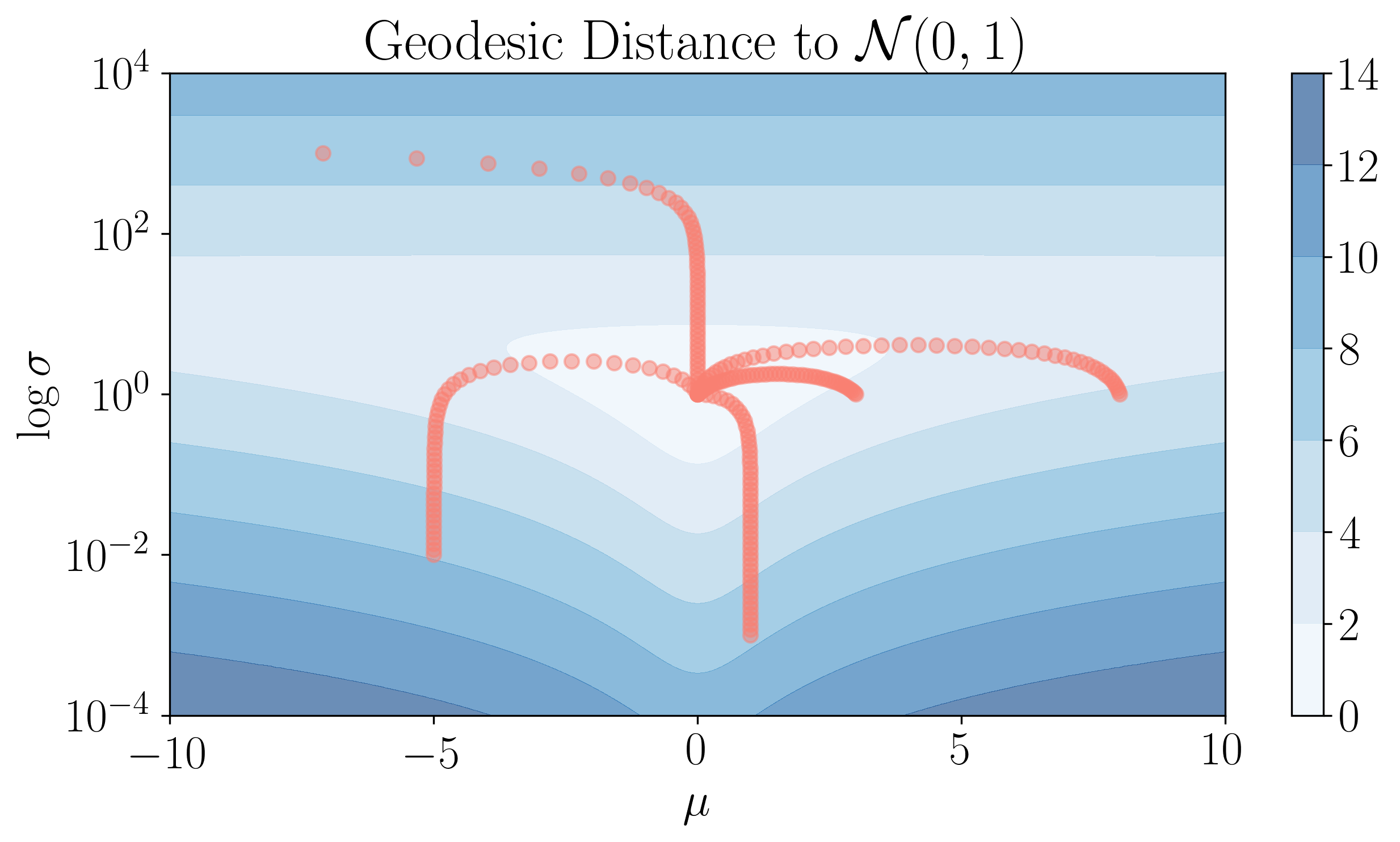
Thanks to the amazing geomstats package, we can visualize in coordinates easily. The idea is by visualizing the contours of the distances from points in to , i.e. corresponding to —the standard normal.

Above, red points are the discretized steps of geodesics from to other Gaussians with different mean and variance. Indeed, geodesics of behave similarly like in the Poincaré half-space model—one of the poster children of the hyperbolic geometry.