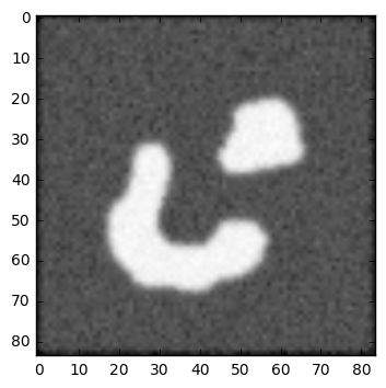
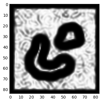
Level Set Method Part II: Image Segmentation

Last post, we looked at the intuition and the formulation of Level Set Method. It’s useful to create a physical simulation like front propagation, e.g. wave simulation, wildfire simulation, or gas simulation. In this post, we are going to see into Level Set Method application in Computer Vision, to solve image segmentation problem.

Image Segmentation with Level Set Method

Recall that the Level Set PDE that we have derived in the last post is as follows:

Here, would need our special attention, as the key to adapting Level Set Method into new problem is by formulating this term. is intuitively a force that drive curve propagation. In other words, we could think of as a velocity field, i.e. is a vector field where at every point it tells us the direction and magnitude of movement of our surface .

As we want to segment an image, then we need to derive from the image. Let’s say we have this image:

As is a velocity field and consider the Level Set PDE above, we want to be high at all region that are not the border of the object we want to segment, and low otherwise. Intuitively, we want the curve to propagate quickly in the background of the image, and we want the curve to slowly propagate or even stop the propagation at the border of the object.

One way to do it is obviously derive our from edge detector. Simplest way to do edge detection is to take the gradients of the image:

So, we could implement it with the code below:

import numpy as np
import scipy.ndimage
import scipy.signal
import matplotlib.pyplot as plt
from skimage import color, io

def grad(x):
    return np.array(np.gradient(x))

def norm(x, axis=0):
    return np.sqrt(np.sum(np.square(x), axis=axis))

def stopping_fun(x):
    return 1. / (1. + norm(grad(x))**2)

img = io.imread('twoObj.bmp')
img = color.rgb2gray(img)
img = img - np.mean(img)

# Smooth the image to reduce noise and separation between noise and edge becomes clear
img_smooth = scipy.ndimage.filters.gaussian_filter(img, sigma)

F = stopping_fun(img_smooth)

So that’s it, we have our . We could plug it into the PDE directly then:

def default_phi(x):
    # Initialize surface phi at the border (5px from the border) of the image # i.e. 1 outside the curve, and -1 inside the curve
    phi = np.ones(x.shape[:2])
    phi[5:-5, 5:-5] = -1.
    return phi

dt = 1.

for i in range(n_iter):
    dphi = grad(phi)
    dphi_norm = norm(dphi)
    dphi_t = F * dphi_norm
    phi = phi + dt * dphi_t

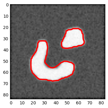
And here’s the segmentation result after several iteration:

This is the naive method for Level Set image segmentation. We could do better by using more complicated formulation for .

Geodesic Active Contour

In Geodesic Active Contour (GAC) formulation of Level Set Method, we define the force as:

The first term is the smoothing term, it moves the curve into the direction of its curvature. The second term is the balloon term, controlling the speed of the curve propagation with parameter . Lastly, the third term is the image attachment term that helps the curve to converge.

def curvature(f):
    fy, fx = grad(f)
    norm = np.sqrt(fx**2 + fy**2)
    Nx = fx / (norm + 1e-8)
    Ny = fy / (norm + 1e-8)
    return div(Nx, Ny)

def div(fx, fy):
    fyy, fyx = grad(fy)
    fxy, fxx = grad(fx)
    return fxx + fyy

def dot(x, y, axis=0):
    return np.sum(x * y, axis=axis)

v = 1.
dt = 1.

g = stopping_fun(img_smooth, alpha)
dg = grad(g)

for i in range(n_iter):
    dphi = grad(phi)
    dphi_norm = norm(dphi)
    kappa = curvature(phi)

    smoothing = g * kappa * dphi_norm
    balloon = g * dphi_norm * v
    attachment = dot(dphi, dg)

    dphi_t = smoothing + balloon + attachment

    phi = phi + dt * dphi_t

Finally, here’s the result of using GAC formulation of Level Set Method for segmenting the same image above:

Notice that qualitatively the segmentation result is better than before, i.e. smoother and better fit.

Conclusion

In this post we looked into the application of Level Set Method on Computer Vision problem, that is image segmentation. We saw the intuition on applying it for image segmentation. We also saw the example of implementation of it. Finally we saw the more complicated formulation, i.e. GAC, for better segmentation.

References

Richard Szeliski. 2010. Computer Vision: Algorithms and Applications (1st ed.). Springer-Verlag New York, Inc., New York, NY, USA.