Level Set Method Part I: Introduction

Looking at the trend in Computer Vision, people steadily abandon the classical methods and just throw everything into Deep Neural Network. It is, however, very useful to study the classical CV method as it is still the key foundation, regardless whether we plan to use DNN or not.

We will look at one of the classic algorithms in Computer Vision: the Level Set Method (LSM). In this post we will see the motivation behind it, the intuition, formulation and finally the implementation of LSM. In the next post, we will apply this method for image segmentation.

Intuition

Let’s say we throw a stone into the middle of a pond. What would happen? There would be a ripple of water (for simplicity let’s just pick one wave), moving from the epicenter, going wide until it dissipates or hit the pond’s edge. How do we model and simulate that phenomenon?

We could do this: model the curve of that ripple and track its movement. Let’s say at time , this is how the ripple looks like:

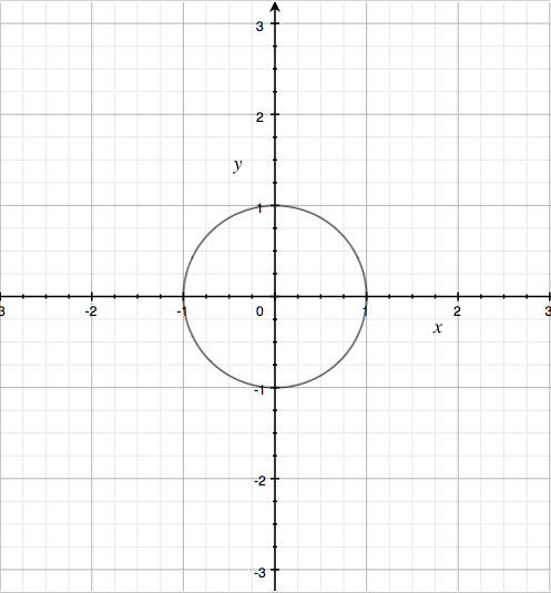
Now, we want to model the movement as time goes. To do that, we have to track the movement of the curve above. One way to do it is to sample sufficient points in that curve and move it to the direction normal to the curve.

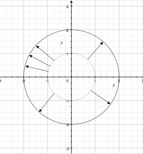
This is a good solution for a very simple simulation (like this one). However, consider what happen to this case:

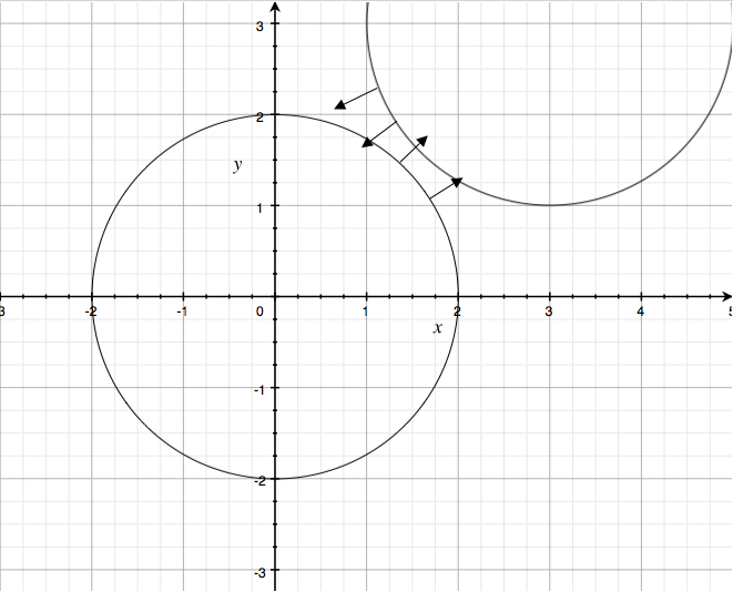
Assuming there’s no external force, those two curve will merge together into a single curve. Also, we have to consider the case when a curve splitting into two or more curves. How do we model that?

This is where LSM shines. Instead of modeling the curve explicitly, LSM will model it implicitly. But how can it help us to model the split, merge, and the movement of the curve, we would ask. Let’s see how it works.

Suppose we have this 3D curve (surface):

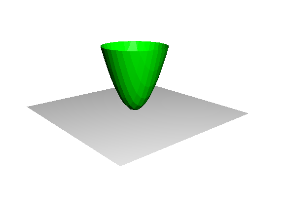
We can model the above curve (circle) with this curve by exploiting the relation between surface, plane, and curve. What we’re going to do is to adjust our surface so that it intersect with a plane in a certain height. Like this:

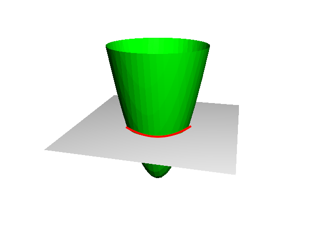
Take at a closer look at the intersection. What is it? It is none other than a curve, specifically, a circle! The curve is the level curve, i.e., a curve of a level set. This is the idea behind LSM. We implicitly modify our curve by transforming the surface then intersecting it to a plane and evaluate the resulting level curve.

But it’s still not clear how do LSM could model the merge and split operation of curves. Let’s do something to our surface and see what does it do to our level curve.

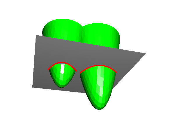
In the above graph, we transform the surface into a surface with two minima. We can see the implication at the level curve, instead of a single circle, now it becomes two. Similarly with merge operation:

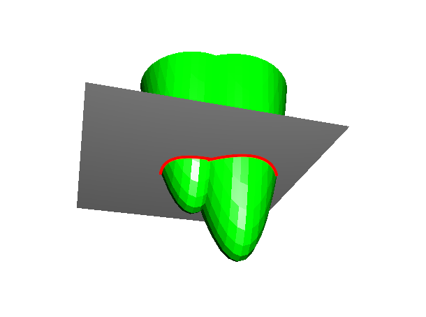
Effortlessly, the level curve captures it!

This is a powerful insight and we’re going to formulate this.

Level Set Method Formulation

Suppose we have surface . The c-level set of this surface is given by:

Formally, we want to track the level curve at , which is the zero level set of .

As we’re dealing with curve and surface evolution, we will parameterized our surface with a temporal variable such that:

We could think of that as the surface at time , given the variable at time .

Next, as we want to track the movement of the zero level curve of , we will derive it with respect to i.e. we derive the equation of motion of . Remember, the derivation of position is speed, and knowing the speed, we could model the movement of the surface.

Using chain rule, we get:

Remember, by definition, the left most partial derivate is the gradient of our surface. And also, for clearer reading we will switch the Leibniz into more compact notation.

As we state above, the direction of the curve’s movement is normal, which is . Of course there would also be a force that move the curve, we call it as . Hence, the speed vector is given by .

Finally, organizing things a little bit, we have our level set equation:

This gives us the speed of the surface evolution of .

Solving the PDE

Knowing the initial value of (let’s say 0 everywhere) and the speed of evolution, we can solve the equation of motion. That is, we want to know surface at time . This is a Partial Differential Equation (PDE).

The simplest way to solve this would be to use Finite Difference Method. Let’s consider forward difference scheme.

Plugging in our we have:

To make it clearer for those who has a background in Machine Learning, recall gradient descent. The update rule is in the form of:

Which is analogous to the finite difference scheme above. So we’re practically doing gradient descent on with respect to !

So that’s it. We just need to provide initial value for and figure out the equation of force , which depend on the system we’re going to model.

Implementation

Given the finite difference formulation to solve the LSM’s PDE, we could now implement it.

As we see, first we need to provide initial values. Then at every iteration, we look at the zero level set of , and we get our curve evolution! For example in Python using matplotlib, it would be something like this:

import numpy as np
import matplotlib.pyplot as plt

phi = np.random.randn(20, 20) # initial value for phi
F = ... # some function
dt = 1
it = 100

for i in range(it):
    dphi = np.gradient(phi)
    dphi_norm = np.sqrt(np.sum(dphi**2, axis=0))

    phi = phi + dt * F * dphi_norm

    # plot the zero level curve of phi
    plt.contour(phi, 0)
    plt.show()

As we can see, the core of LSM could be implemented with just a few lines of code. Bear in mind, this is the simplest formulation of LSM. There are many sophisticated variations of LSM which modifies .

Conclusion

In this post, we looked at Level Set Method (LSM) which is a method to model curve evolution using implicit contour. LSM is powerful because we don’t have to explicitly model difficult curve evolution like merge and split directly.

Then, we looked at the LSM formulation and how to solve the LSM as PDE using Finite Difference Method.

Finally, we implemented the simplest formulation of LSM in Python.

References

Richard Szeliski. 2010. Computer Vision: Algorithms and Applications (1st ed.). Springer-Verlag New York, Inc., New York, NY, USA.
http://step.polymtl.ca/~rv101/levelset/