Least Squares GAN

Thanks to F-GAN, which established the general framework of GAN training, recently we saw modifications of GAN which unlike the original GAN, learn other metrics other than Jensen-Shannon divergence (JSD).

One of those modifications are Wasserstein GAN (WGAN), which replaces JSD with Wasserstein distance. It works wonderfully well and even the authors claimed that it cures the mode collapse problem and providing GAN with meaningful loss function. Although the implementation is quite straightforward, the theory behind WGAN is heavy and requires some “hack” e.g. weight clipping. Moreover, the training process and the convergence are slower than the original GAN.

Now, the question is: could we design GAN that works well, fast, simpler, and more intuitive compared to WGAN?

The answer yes. What we need is to back to basic.

Least Squares GAN

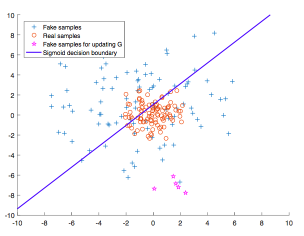
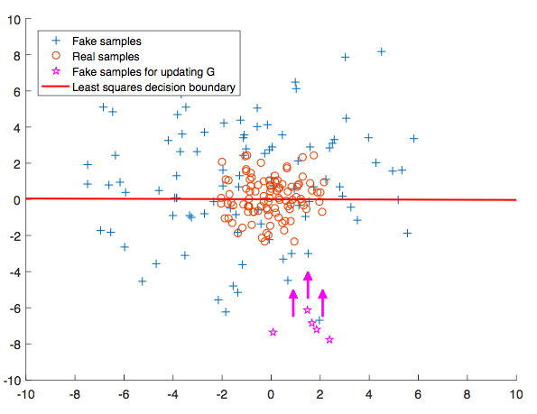
The main idea of LSGAN is to use loss function that provides smooth and non-saturating gradient in discriminator . We want to “pull” data generated by generator towards the real data manifold , so that generates data that are similar to .

As we know in original GAN, uses log loss. The decision boundary is something like this:

As uses sigmoid function, and as it is saturating very quickly, even for somewhat-still-small data point , it will quickly ignore the distance of to the decision boundary . What it means is that it essentially won’t penalize that is far away from in the manifold. That is, as long as is correctly labeled, we’re happy. Consequently, as becoming bigger and bigger, the gradient of quickly goes down to , as log loss doesn’t care about the distance, only the sign.

For learning the manifold of , then log loss is not effective. Generator is trained using the gradient of . If the gradient of is saturating to , then won’t have the necessary information for learning .

Enter loss:

In loss, data that are quite far away from (in this context, the regression line of ) will be penalized proportional to the distance. The gradient therefore will only become when perfectly captures all of . This will guarantee to yield informative gradients if has not captured the data manifold.

During the optimization process, the only way for loss of to be small is to make generating that are close to . This way, will actually learn to match !

The overall training objective of LSGAN then could be stated as follows:

Above, we choose to state that it’s the real data. Conversely, we choose as it the fake data. Finally , as we want to fool .

Those values is not the only valid values, though. The authors of LSGAN provides some theory that optimizing the above loss is the same as minimizing Pearson divergence, if and . Hence, choosing is equally valid.

Our final loss is as follows:

LSGAN implementation in Pytorch

Let’s outline the modifications done by LSGAN to the original GAN:

1. Remove from
2. Use loss instead of log loss

So let’s begin by doing the the first checklist:

G = torch.nn.Sequential(
    torch.nn.Linear(z_dim, h_dim),
    torch.nn.ReLU(),
    torch.nn.Linear(h_dim, X_dim),
    torch.nn.Sigmoid()
)

D = torch.nn.Sequential(
    torch.nn.Linear(X_dim, h_dim),
    torch.nn.ReLU(), # No sigmoid
    torch.nn.Linear(h_dim, 1),
)

G_solver = optim.Adam(G.parameters(), lr=lr)
D_solver = optim.Adam(D.parameters(), lr=lr)

The rest is straightforward, following the loss function above.

for it in range(1000000):
    # Sample data
    z = Variable(torch.randn(mb*size, z_dim))
    X, * = mnist.train.next_batch(mb_size)
    X = Variable(torch.from_numpy(X))

    # Dicriminator
    G_sample = G(z)
    D_real = D(X)
    D_fake = D(G_sample)

    # Discriminator loss
    D_loss = 0.5 * (torch.mean((D_real - 1)**2) + torch.mean(D_fake**2))

    D_loss.backward()
    D_solver.step()
    reset_grad()

    # Generator
    G_sample = G(z)
    D_fake = D(G_sample)

    # Generator loss
    G_loss = 0.5 * torch.mean((D_fake - 1)**2)

    G_loss.backward()
    G_solver.step()
    reset_grad()

The full code is available at https://github.com/wiseodd/generative-models.

Conclusion

In this post we looked at LSGAN, which modifies the original GAN by using loss instead of log loss.

We looked at the intuition why loss could help GAN learning the data manifold. We also looked at the intuition on why GAN could not learn effectively using log loss.

Finally, we implemented LSGAN in Pytorch. We found that the implementation of LSGAN is very simple, amounting to just two line changes.

References

1. Nowozin, Sebastian, Botond Cseke, and Ryota Tomioka. “f-GAN: Training generative neural samplers using variational divergence minimization.” Advances in Neural Information Processing Systems. 2016. arxiv
2. Mao, Xudong, et al. “Multi-class Generative Adversarial Networks with the L2 Loss Function.” arXiv preprint arXiv:1611.04076 (2016). arxiv