Let
We must then approximate
The estimate
In the context of Bayesian neural networks, the Laplace approximation (LA) is a family of methods for obtaining a Gaussian approximate posterior distribution of networks’ parameters.
The fact that it produces a Gaussian approximation is a step up from the MAP estimation: particularly, it conveys some notion of uncertainty in
Given the MAP estimate
(Note that the gradient
For simplicity, let
where the equality follows from the fact the integral above is the famous, tractable Gaussian integral. Combining both approximations, we obtain
That is, we obtain a tractable, easy-to-work-with Gaussian approximation to the intractable posterior via a simple second-order Taylor expansion!
Moreover, this is not just any Gaussian approximation: Notice that this Gaussian is fully determined once we have the MAP estimate
Given this approximation, we can then use it as a proxy to the true posterior. For instance, we can use it to obtain the predictive distribution
which in general is less overconfident compared to the MAP-estimate-induced predictive distribution [3].
What we have seen is the most general framework of the LA.
One can make a specific design decision, such as by imposing a special structure to the Hessian
The laplace-torch library
The simplicity of the LA is not without a drawback.
Recall that the parameter
Motivated by this observation, in our NeurIPS 2021 paper titled “Laplace Redux – Effortless Bayesian Deep Learning”, we showcase that (i) the Hessian can be obtained cheaply, thanks to recent advances in second-order optimization, and (ii) even the simplest LA can be competitive to more sophisticated VB and MCMC methods, while only being much cheaper than them.
Of course, numbers alone are not sufficient to promote the goodness of the LA.
So, in that paper, we also propose an extendible, easy-to-use software library for PyTorch called laplace-torch, which is available at this Github repo.
The laplace-torch is a simple library for, essentially, “turning standard NNs into BNNs”.
The main class of this library is the class Laplace, which can be used to transform a standard PyTorch model into a Laplace-approximated BNN.
Here is an example.
from laplace import Laplace
model = load_pretrained_model()la = Laplace(model, 'regression')
# Compute the Hessianla.fit(train_loader)
# Hyperparameter tuningla.optimize_prior_precision()
# Make predictionpred_mean, pred_var = la(x_test)
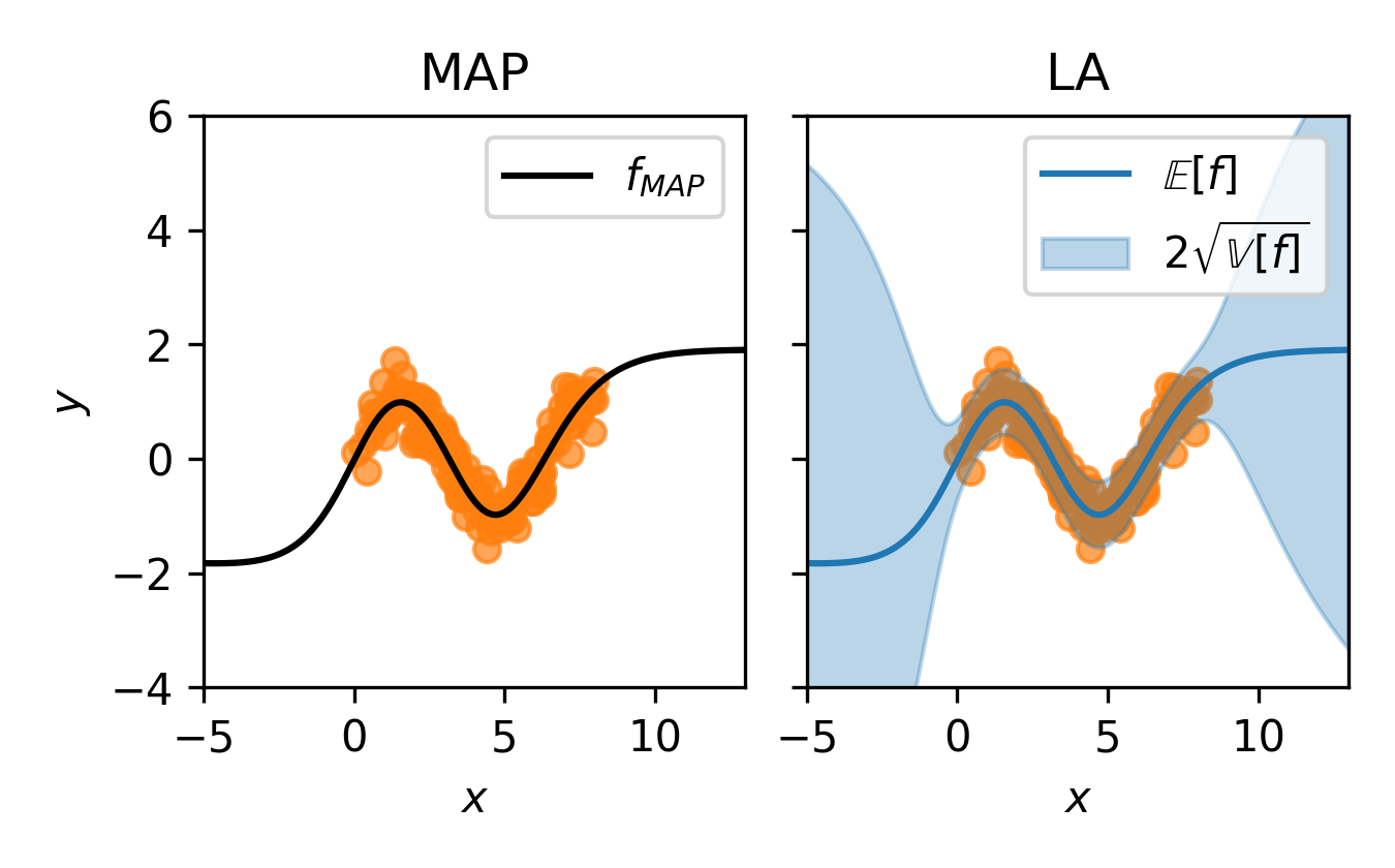
The resulting object, la is a fully-functioning BNN, yielding the following prediction.
(Notice the identical regression curves—the LA essentially imbues MAP predictions with uncertainty estimates.)

Of course, laplace-torch is flexible: the Laplace class has almost all state-of-the-art features in Laplace approximations.
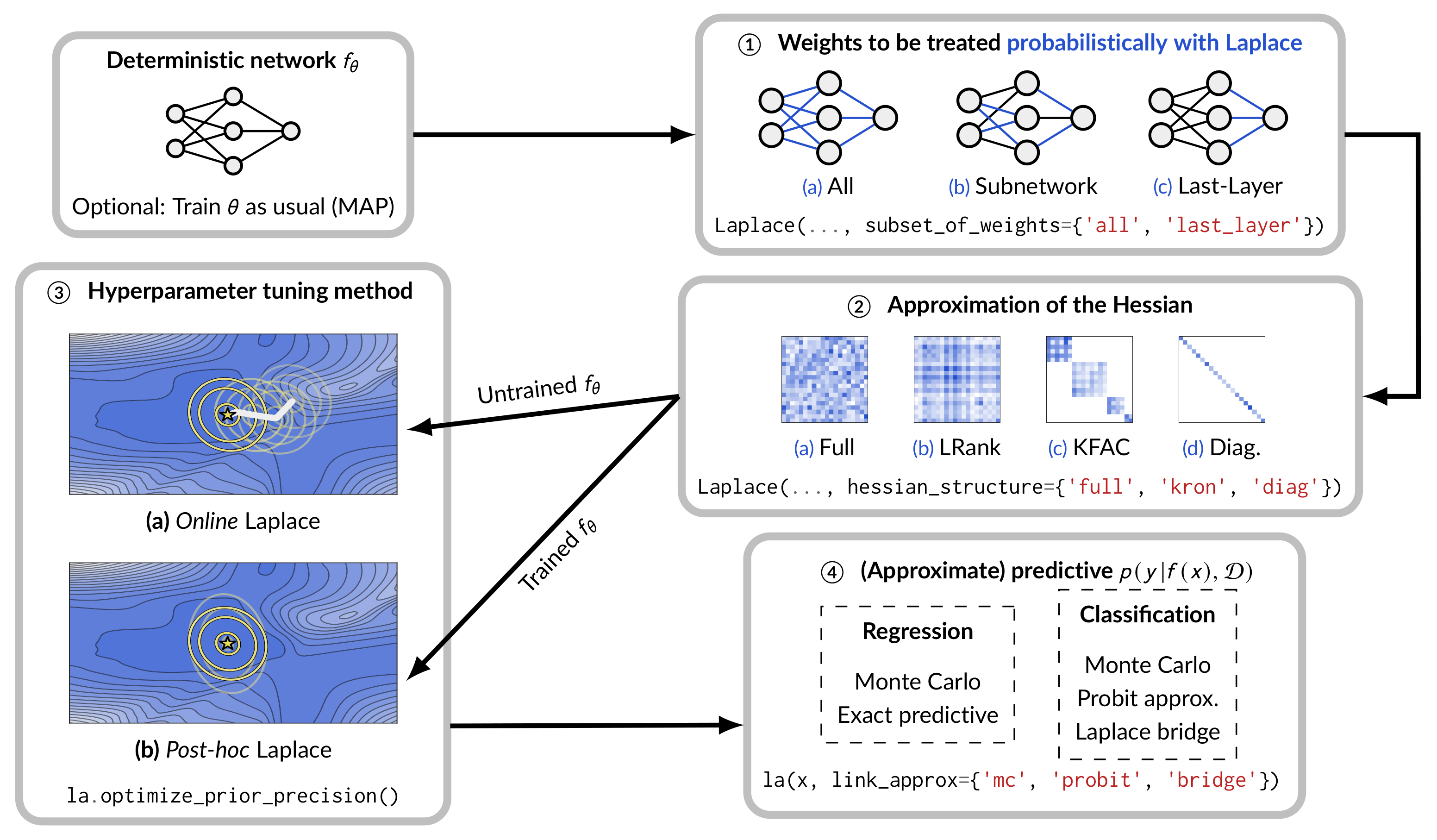
Those features, along with the corresponding options in laplace-torch, are summarized in the following flowchart.
(The options 'subnetwork' for subset_of_weights and 'lowrank' for hessian_structure are in the work, by the time this post is first published.)

The laplace-torch library uses a very cheap yet highly-performant flavor of LA by default, based on [4]:
def Laplace(model, likelihood, subset_of_weights='last_layer', hessian_structure='kron', ...)That is, by default the Laplace class will fit a last-layer Laplace with a Kronecker-factored Hessian for approximating the covariance.
Let us see how this default flavor of LA performs compared to the more sophisticated, recent (all-layer) Bayesian baselines in classification.

Here we can see that Laplace, with default options, improves the calibration (in terms of expected calibration error (ECE)) of the MAP model.
Moreover, it is guaranteed to preserve the accuracy of the MAP model—something that cannot be said for other baselines.
Ultimately, this improvement is cheap: laplace-torch only incurs little overhead relative to the MAP model—far cheaper than other Bayesian baselines.
Hyperparameter Tuning
Hyperparameter tuning, especially for the prior variance/precision, is crucial in modern Laplace approximations for BNNs.
laplace-torch provides several options: (i) cross-validation and (ii) marginal-likelihood maximization (MLM, also known as empirical Bayes and type-II maximum likelihood).
Cross-validation is simple but needs a validation dataset.
In laplace-torch, this can be done via the following.
la.optimize_prior_precision(method='CV', val_loader=val_loader)A more sophisticated and interesting tuning method is MLM.
Recall that by taking the second-order Taylor expansion over the log-posterior, we obtain an approximate normalization constant
In laplace-torch, the marginal likelihood can be accessed via
ml = la.log_marginal_likelihood(prior_precision)This function is compatible with PyTorch’s autograd, so we can backpropagate through it to obtain the gradient of
ml.backward() # Works!Thus, MLM can easily be done in laplace-torch.
By extension, recent methods such as online MLM [5], can also easily be applied using laplace-torch.
Outlooks
The laplace-torch library is continuously developed.
Support for more likelihood functions and priors, subnetwork Laplace, etc. are on the way.
In any case, we hope to see the revival of the LA in the Bayesian deep learning community. So, please try out our library at https://github.com/AlexImmer/Laplace!
References
- Hein, Matthias, Maksym Andriushchenko, and Julian Bitterwolf. “Why ReLU networks yield high-confidence predictions far away from the training data and how to mitigate the problem.” CVPR 2019.
- Laplace, Pierre Simon. “Mémoires de Mathématique et de Physique, Tome Sixieme” 1774.
- MacKay, David JC. “The evidence framework applied to classification networks.” Neural computation 4.5 (1992).
- Kristiadi, Agustinus, Matthias Hein, and Philipp Hennig. “Being Bayesian, even just a bit, fixes overconfidence in ReLU networks.” ICML 2020.
- Immer, Alexander, Matthias Bauer, Vincent Fortuin, Gunnar Rätsch, and Mohammad Emtiyaz Khan. “Scalable marginal likelihood estimation for model selection in deep learning.” ICML, 2021.