In machine learning, especially in neural networks, the Hessian matrix is often treated synonymously with curvatures, in the following sense. Suppose defined by is a (real-valued) neural network, mapping an input to the output under the parameter . Given a dataset , we can define a loss function by such as the mean-squared-error or cross-entropy loss. (We do not explicitly show the dependency of to and for brevity.) Assuming the standard basis for , from calculus we know that the second partial derivatives of at a point form a matrix called the Hessian matrix at .
Often, one calls the Hessian matrix the “curvature matrix” of at [1, 2, etc.]. Indeed, it is well-justified since as we have learned in calculus, the eigenspectrum of this Hessian matrix represents the curvatures of the loss landscape of at . It is, however, not clear from calculus alone what is the precise geometric meaning of these curvatures. In this post, we will use tools from differential geometry—especially the hypersurface theory—to study the geometric interpretation of the Hessian matrix.
Loss Landscapes as Hypersurfaces
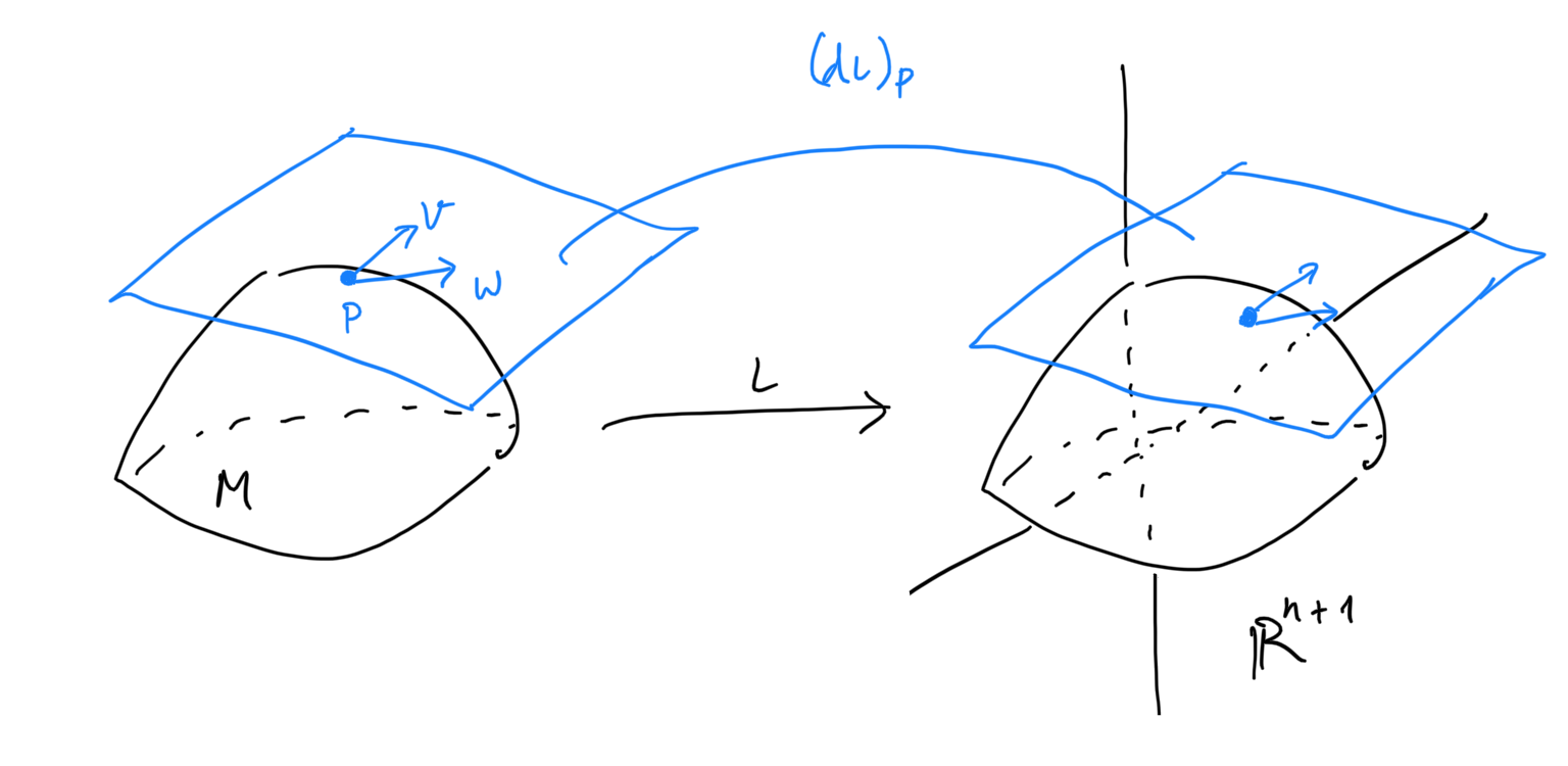
We begin by formalizing what exactly is a loss landscape via the Euclidean hypersurface theory. We call an -dimensional manifold a (Euclidean) hypersurface of if is a subset of (equipped with the standard basis) and the inclusion is a smooth topological embedding. Since is equipped with a metric in the form of the standard dot product, we can equip with an induced metric characterized at each point by
for all tangent vectors . Here, represents the dot product and is the differential of at which is represented by the Jacobian matrix of at . In matrix notation this is
Intuitively, the induced inner product on at is obtained by “pushing forward” tangent vectors and using the Jacobian at and compute their dot product on .
Fig. Pushforward.
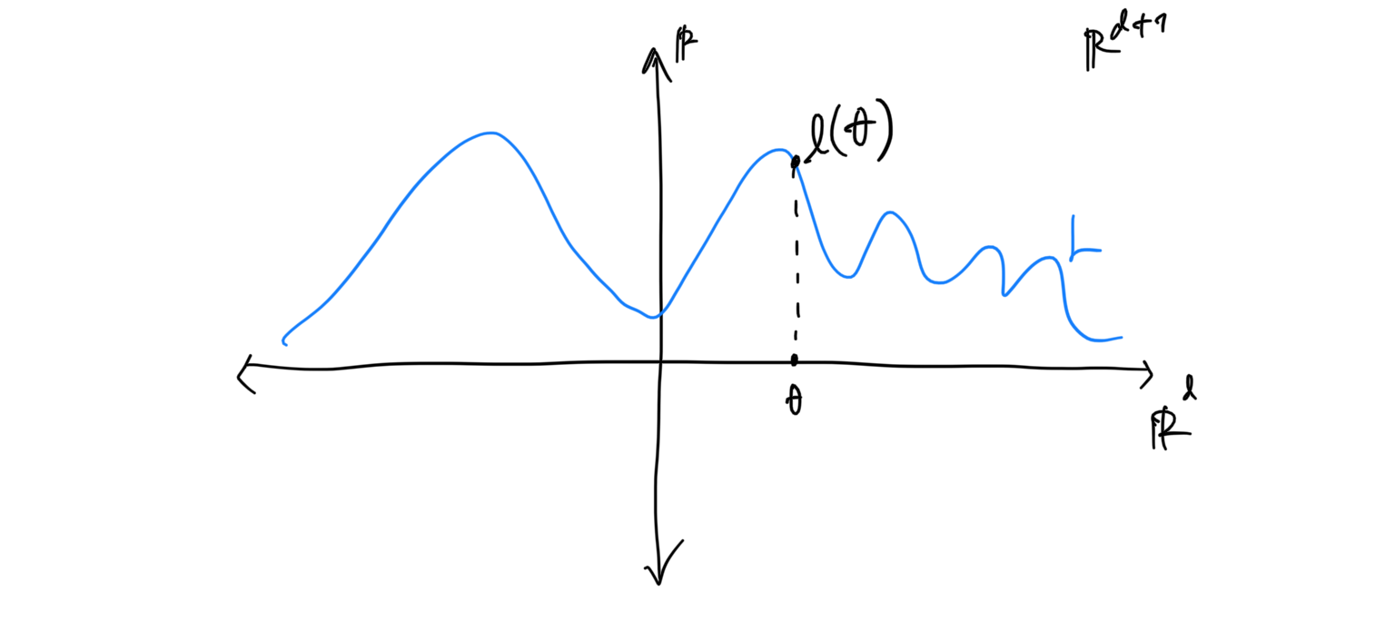
Let is a smooth real-valued function over an open subset , then the graph of is the subset which is a hypersurface in . In this case, we can describe via the so-called graph parametrization which is a function defined by .
Coming back to our neural network setting, assuming that the loss is smooth, the graph is a Euclidean hypersurface of with parametrization defined by . Furthermore, the metric of is given by the Jacobian of the parametrization and the standard dot product on , as before. Thus, the loss landscape of can indeed be amenable to geometric analysis.
Fig. The graph of a function as a hypersurface.
The Second Fundamental Form and Shape Operator
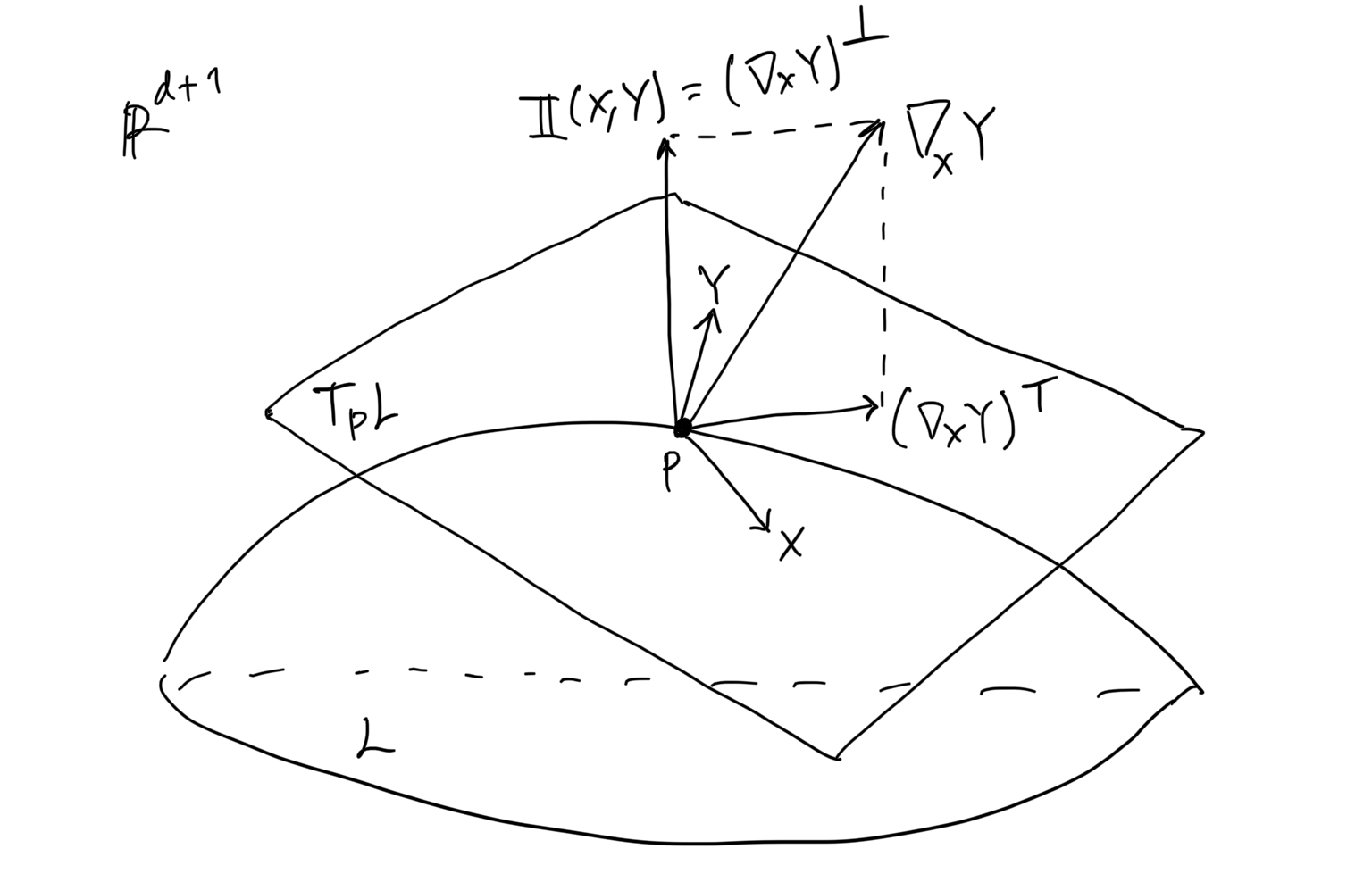
Consider vector fields and on the hypersurface . We can view them as vector fields on and thus the directional derivative on is well-defined at all points in . That is, at every , is a -dimensional vector “rooted” at . This vector can be decomposed as follows:
where and are the orthogonal projection operators onto the tangent/normal space of at . We define the second fundamental form as the map that takes two vector fields on and yielding normal vector fields of , as follows:
See the following figure for an intuition.
Fig. The second fundamental form.
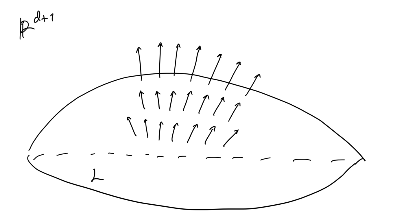
Since is a -dimensional hypersurface of -dimensional Euclidean space, the normal space at each point of has dimension one, and there exist only two ways of choosing a unit vector field normal to . Any choice of the unit vector field thus automatically gives a basis for for all . One of the choices is the following normal vector field which is oriented outward relative to .
Fig. A unit normal vector field.
Another choice is the same unit normal field but oriented inward relative to .
Fix a unit normal field . We can replace the vector-valued second fundamental form with a simpler scalar-valued form. We define the scalar second fundamental form of to be
Furthermore, we define the shape operator of as the map , mapping a vector field to another vector field on , characterized by
Based on the characterization above, we can alternatively view as an operator obtained by raising an index of , i.e. multiplying the matrix of with the inverse-metric.
Note that, at each point , the shape operator at is a linear endomorphism of , i.e. it defines a map from the tangent space to itself. Furthermore, we can show that and thus is symmetric. This implies that is self-adjoint since we can write
Altogether, this means that at each , the shape operator at can be represented by a symmetric matrix.
Principal Curvatures
The previous fact about the matrix of says that we can apply eigendecomposition on and obtain real eigenvalues and an orthonormal basis for formed by the eigenvectors corresponding to these eigenvalues. We call these eigenvalues the principal curvatures of at and the corresponding eigenvectors the principal directions. Moreover, we also define the Gaussian curvature as and the mean curvature as .
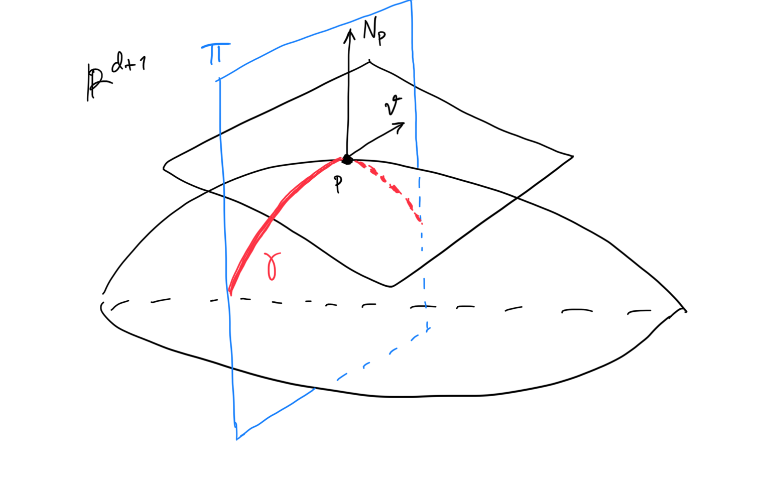
Fig. Principal curvatures.
The intuition of the principal curvatures and directions in is shown in the preceding figure. Suppose is a surface in . Choose a tangent vector . Together with the choice of our unit normal vector at , we obtain a plane passing through . The intersection of and the neighborhood of in is a plane curve containing . We can now compute the curvature of this curve at as usual, in the calculus sense (the reciprocal of the radius of the osculating circle at ). Then, the principal curvatures of at are the minimum and maximum curvatures obtained this way. The corresponding vectors in that attain the minimum and maximum are the principal directions.
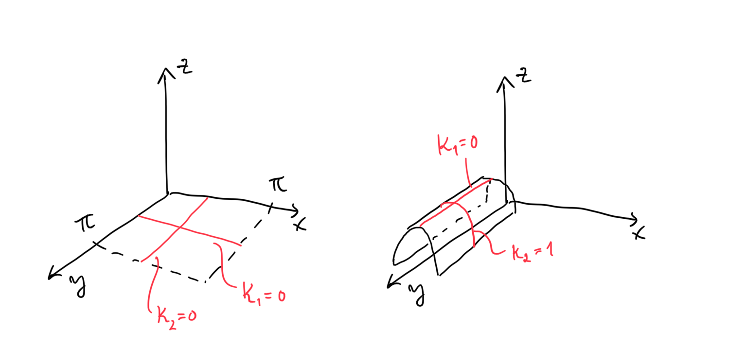
Principal and mean curvatures are not intrinsic to a hypersurface. There are two hypersurfaces that are isometric, but have different principal curvatures and hence different mean curvatures. Consider the following two surfaces.
Fig. Principal curvatures are extrinsic.
The first (left) surface is the plane described by the parametrization for and . The second one is the half cylinder for and . It is clear that they have different principal curvatures since the plane is a flat while the half-cylinder is “curvy”. Indeed, assuming a downward pointing normal, we can see that for the plane and for the half-cylinder and thus their mean curvatures differ. However, they are actually isometric to each other—from the point of view of Riemannian geometry, they are the same. Thus, both principal and mean curvatures depend on the choice of the parametrization and not intrinsic.
Remarkably, the Gaussian curvature is intrinsic: All isometric hypersurfaces of dimension have the same Gaussian curvature (up to sign). Using the previous example: the plane and half-cylinder have the same Gaussian curvature of . In 2D surfaces, this is a classic result which Gauss named Theorema Egregium. For hypersurfaces with dimension , it can be shown that the Gaussian curvature is intrinsic up to sign [5, Ch. 7, Cor. 23].
The Loss Landscape’s Hessian
Now we are ready to draw a geometric connection between principal curvatures and the Hessian of . Let be graph parametrization of the loss landscape . The coordinates thus give local coordinates for . The coordinate vector field , push forward to vector fields on , via the Jacobian of . At each , these vector fields form a basis for , viewed as a collection of vectors in .
If we think of as a vector-valued function of , then by definition of Jacobian, these push-forwarded coordinate vector fields can be written for every as
for each .
Let us suppose we are given a unit normal field to . Then we have the following result.
Proposition 1.Suppose is the loss landscape of , is the graph parametrization of . Suppose further that are the vector fields determined by which restriction at each is a basis for , and suppose is a unit normal field on . Then the scalar second fundamental form is given by
Where is the last component of the unit normal field.
Proof. To show the first equality, one can refer to Proposition 8.23 in [1], which works for any parametrization and not just the graph parametrization. Now recall that . Therefore for each :
and thus
Taking the inner product with the unit normal field , we obtain
where is the -st component function (it is a function ) of the normal field . At each , the matrix of is therefore times the Hessian matrix of at .
Finally, we show the connection between the principal curvatures with the scalar second fundamental form, and hence the principal curvatures with the Hessian. The following proposition says that at a critical point, the unit normal vector can be chosen as and thus the scalar second fundamental form coincides with the Hessian of . Furthermore, by orthonormalizing the basis for the tangent space at that point, we can show that the matrix of the scalar second fundamental form in this case is exactly the matrix of the shape operator at and thus the Hessian encodes the principal curvatures at that point.
Proposition 2. _Suppose is a loss landscape with its graph parametrization and let \theta__ \in \R^d be a critical point of and p\__ := (\theta*\*^1, \dots, \theta*_^d, \ell(\theta\__)) \in L. Then the matrix of the shape operator of at is equal to the Hessian matrix of at ._
Proof. We can assume w.l.o.g. that the basis for is orthonormal by applying the Gram-Schmidt algorithm on linearly independent tangent vectors in . Furthermore pick as the choice of the unit normal at . We can do so since by hypothesis is a critical point and therefore is perpendicular to .
It follows by Proposition 1 that the matrix of the scalar second fundamental form of at is equal to the Hessian matrix of at . Moreover, since we have an orthonormal basis for , the metric of at is represented by the diagonal matrix. This implies that the matrix of the shape operator at is equal to the matrix of the second fundamental form and the claim follows directly.
As a side note, we can actually have a more general statement: At any point in a hypersurface with any parametrization, the principal curvatures give a concise description of the local shape of the hypersurface by approximating it with the graph of a quadratic function. See Prop. 8.24 in [3] for a detailed discussion.
Flatness and Generalization
In deep learning, there have been interesting works connecting the “flatness” of the loss landscape’s local minima with the generalization performance of an NN. The conjecture is that the flatter a minimum is, the better the network generalizes. “Flatness” here often refers to the eigenvalues or trace of the Hessian matrix at the minima. However, this has been disputed by e.g. [4] and rightly so.
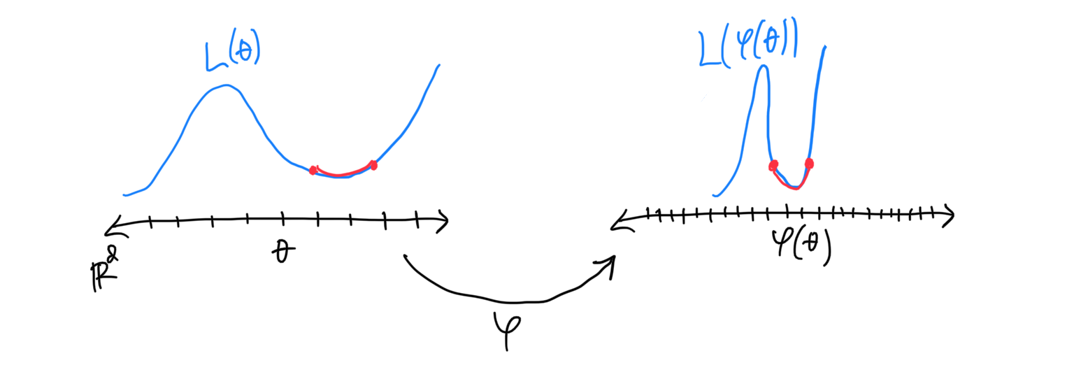
As we have seen previously, at a minimum, the principal and mean curvature (the eigenvalues and trace of the Hessian of , resp.) are not intrinsic. Different parametrization of can yield different principal and mean curvatures. Just like the illustration with the plane and the half-cylinder above, [4] illustrates this directly in the loss landscape. In particular, we can apply a bijective transformation to the original parameter space s.t. the resulting loss landscape is isometric to the original loss landscape and the particular minimum does not change, i.e. . See the following figure for an illustration (we assume that the length of the red curves below is the same).
Fig. Principal curvatures are not invariant under reparametrization.
It is clear that the principal curvature changes even though functionally, the NN still represents the same function. Thus, we cannot actually connect the notion of “flatness” that are common in literature to the generalization ability of the NN. A definitive connection between them must start with some intrinsic notion of flatness—for starter, the Gaussian curvature, which can be easily computed since it is just the determinant of the Hessian at the minima.
References
Martens, James. “New Insights and Perspectives on the Natural Gradient Method.” arXiv preprint arXiv:1412.1193 (2014).
Dangel, Felix, Stefan Harmeling, and Philipp Hennig. “Modular Block-diagonal Curvature Approximations for Feedforward Architectures.” AISTATS. 2020.
Lee, John M. Riemannian manifolds: an introduction to curvature. Vol. 176. Springer Science & Business Media, 2006.
Dinh, Laurent, et al. “Sharp Minima can Generalize for Deep Nets.” ICML, 2017.
Spivak, Michael D. A comprehensive introduction to differential geometry. Publish or perish, 1970.