/ 5 min read
Gaussian Anomaly Detection
Suppose you are a teacher in kindergarten. Looking at your class, it seems there are a few children that are out of the ordinary, in term of their height compared to the rest of the class. It seems that they are different, by just looking at them, you’re sure of it. You’ve talked about this to your principle: “Hey, A and B in my class are way taller than the rest of the class”. The principle replied: “You sure it’s not just an optical illusion? Could you present me with a proof?“. You are then wondering, is there any method that can help you identifying those children?
Yes, there is! It’s called Anomaly Detection!
Specifically, what we’re going to do is Gaussian Anomaly Detection, because we’ll assume that our data are normally distributed, and fit it into a Gaussian distribution. Recall, a Gaussian is a distribution that is paramaterized by two values: mean and standard deviation.
But, what does it mean to fit data into a Gaussian distribution? Well, it means that we want to find a Gaussian that best represents our data by finding the optimal parameters (mean and standard deviation) under our data. Now, from here, we have two methods for finding the optimal parameters for the Gaussian, by using Frequentist or Bayesian method. Let’s go with Frequentist method first.
Frequentist Method
In a Frequentist setting, finding the optimal parameter equals to finding the parameter that maximize the likelihood of the data. There are two laws that are supporting this method: the Likelihood Principle, and the Law of Likelihood. Basically, they say that “the parameter value which maximizes the likelihood function is the value which is most strongly supported by the evidence”.
Now, how do we calculate the maximum likelihood? It turns out, the Maximum Likelihood Estimation (MLE) of mean and standard deviation of a Gaussian are just their sample mean and sample standard deviation. I’m not going to derive it here, but you could read the Bishop’s book to understand why it’s just sample mean and sample standard deviation.
So, let’s say we have these data:
X = np.array([10, 14, 12, 1200, 25, 120, 54, 32, 18, 23])The best fit Gaussian for those data is N(mu_MLE, std_MLE), that is, Gaussian parameterized by the maximum likelihood estimation of its parameters.
mu = np.mean(X) # 150.8sigma = np.std(X) # 351.1199So, that’s it! We’ve fitted our data into N(150.8, 351.1199)!

Now, what’s left is the evaluation phase. We want to know, based our Gaussian, whether or not a new data is an anomaly. To do that, we need a threshold value that says, if the probability of the new data under our Gaussian is higher or lower than the threshold, it’s probably an anomaly.
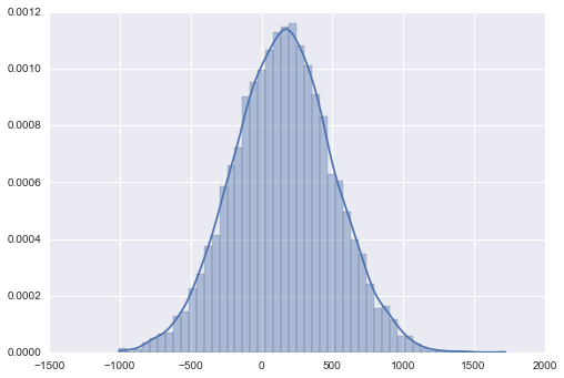
We could intuitively define the threshold by looking at the plot of our Gaussian above. The anomalies would be the data that fall under the low probability areas of the Gaussian, because being in the low probability area, that data is highly unlikely to be distributed in our distribution. Those low probability areas are the left and the right tails of the Gaussian. So, we could say that, for example, 25% area under the tails are the anomaly regions.
# Thresholds: 25 percent of left tail and 25 percent of right tailt1, t2 = 25, 75
# Our test dataX_test = np.array([1500, 10, 35, 400])
# Use CDF to find the position of the data under the curvey_test = st.norm.cdf(X_test, mu, sigma)
# Compare the CDFs with the thresholdsfor y in y_test:    if y < t1 or y > t2:        print 'Anomaly!'
Bayesian Method
We could also use Bayesian method to fit the Gaussian. The obvious advantage of Bayesian method is that it will not just provide a point estimate of the parameters we want to find. Bayesian method will model our parameters as distributions, so we get whole range of all possible values of those parameters, and we can do more with it.
For this, I will use Python library called PyMC. First of all, we need to specify a prior for all of the parameters we want to find: mean and standard deviation. Pretend that I know nothing about those parameters, so the logical choice of prior will be Uniform prior.
# Priormu = pymc.Uniform('mu', 0, 1000)sigma = pymc.Uniform('sigma', 0, 1000)Now, we need to express our data in term of likelihood function. Because we’re assuming the normality of our data, we will use Gaussian likelihood function. And because we already have our data X, we will set this as observed=True.
# Likelihoodlikelihood = pymc.Normal('likelihood', mu, sigma**-2, observed=True, value=X)The only thing left is to infer the posterior distribution of our mean and standard deviation.
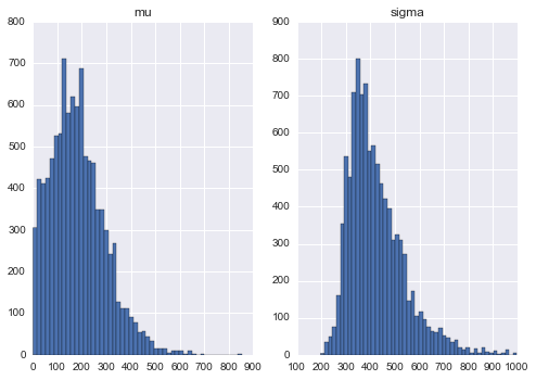
mcmc = pymc.MCMC([mu, sigma, likelihood])mcmc.sample(iter=11000, burn=1000)Here’s our posterior distributions obtained after 11000 MCMC iteration:

As you can see, we get a distribution, not just a point estimate for our parameters. That means, we can do a lot more analysis to these result compared to MLE result. For now though, we will just take a point estimate of mean and standard deviation, just like MLE. Because the distributions are rather skewed, we will use median as our point estimates.
mu = stats['mu']['quantiles'][50] # 171.0512sigma = stats['sigma']['quantiles'][50] # 398.2883Now, we could just plug those parameters to the Gaussian, and we get our fitted Gaussian distribution. Using the same idea, you could determine whether a new data point is an anomaly or not.