/ 6 min read
Generative Adversarial Nets in TensorFlow
Generative Adversarial Nets, or GAN in short, is a quite popular neural net. It was first introduced in a NIPS 2014 paper by Ian Goodfellow, et al. This paper literally sparked a lot of interest in adversarial training of neural net, proved by the number of citation of the paper. Suddenly, many flavors of GAN came up: DCGAN, Sequence-GAN, LSTM-GAN, etc. In NIPS 2016, there will even be a whole workshop dedicated for adversarial training!
Note, the code is available in https://github.com/wiseodd/generative-models.
First, let’s review the main points about the paper. After that, as always, we will try to implement GAN using TensorFlow, with MNIST data.
Generative Adversarial Nets
Let’s consider the rosy relationship between a money conterfeiting criminal and a cop. What’s the objective of the criminal and what’s the objective of the cop in term of counterfeited money? Let’s enumerate:
- To be a successful money counterfeiter, the criminal wants to fool the cop, so that the cop can’t tell the difference between counterfeited money and real money
- To be a paragon of justice, the cop wants to detect counterfeited money as good as possible
There, we see we have a clash of interest. This kind of situation could be modeled as a minimax game in Game Theory. And this process is called Adversarial Process.
Generative Adversarial Nets (GAN), is a special case of Adversarial Process where the components (the cop and the criminal) are neural net. The first net generates data, and the second net tries to tell the difference between the real data and the fake data generated by the first net. The second net will output a scalar [0, 1] which represents a probability of real data.
In GAN, the first net is called Generator Net

At the equilibrium point, which is the optimal point in minimax game, the first net will models the real data, and the second net will output probability of 0.5 as the output of the first net = real data.
“BTW why do we interested in training GAN?” might come in mind. It’s because probability distribution of data
GAN Implementation
By the definition of GAN, we need two nets. This could be anything, be it a sophisticated net like convnet or just a two layer neural net. Let’s be simple first and use a two layer nets for both of them. We’ll use TensorFlow for this purpose.
# Discriminator NetX = tf.placeholder(tf.float32, shape=[None, 784], name='X')
D_W1 = tf.Variable(xavier_init([784, 128]), name='D_W1')D_b1 = tf.Variable(tf.zeros(shape=[128]), name='D_b1')
D_W2 = tf.Variable(xavier_init([128, 1]), name='D_W2')D_b2 = tf.Variable(tf.zeros(shape=[1]), name='D_b2')
theta_D = [D_W1, D_W2, D_b1, D_b2]
# Generator NetZ = tf.placeholder(tf.float32, shape=[None, 100], name='Z')
G_W1 = tf.Variable(xavier_init([100, 128]), name='G_W1')G_b1 = tf.Variable(tf.zeros(shape=[128]), name='G_b1')
G_W2 = tf.Variable(xavier_init([128, 784]), name='G_W2')G_b2 = tf.Variable(tf.zeros(shape=[784]), name='G_b2')
theta_G = [G_W1, G_W2, G_b1, G_b2]
def generator(z):    G_h1 = tf.nn.relu(tf.matmul(z, G_W1) + G_b1)    G_log_prob = tf.matmul(G_h1, G_W2) + G_b2    G_prob = tf.nn.sigmoid(G_log_prob)    return G_prob
def discriminator(x):    D_h1 = tf.nn.relu(tf.matmul(x, D_W1) + D_b1)    D_logit = tf.matmul(D_h1, D_W2) + D_b2    D_prob = tf.nn.sigmoid(D_logit)    return D_prob, D_logit
Above, generator(z) takes 100-dimensional vector and returns 786-dimensional vector, which is MNIST image (28x28). z here is the prior for the
The discriminator(x) takes MNIST image(s) and return a scalar which represents a probability of real MNIST image.
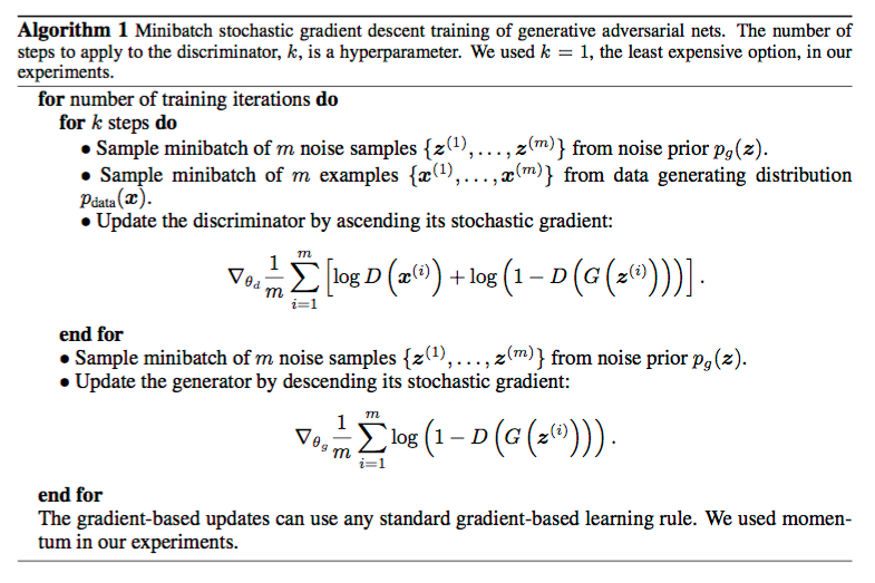
Now, let’s declare the Adversarial Process for training this GAN. Here’s the training algorithm from the paper:

G_sample = generator(Z)D_real, D_logit_real = discriminator(X)D_fake, D_logit_fake = discriminator(G_sample)
D_loss = -tf.reduce_mean(tf.log(D_real) + tf.log(1. - D_fake))G_loss = -tf.reduce_mean(tf.log(D_fake))
Above, we use negative sign for the loss functions because they need to be maximized, whereas TensorFlow’s optimizer can only do minimization.
Also, as per the paper’s suggestion, it’s better to maximize tf.reduce_mean(tf.log(D_fake)) instead of minimizing tf.reduce_mean(1 - tf.log(D_fake)) in the algorithm above.
Then we train the networks one by one with those Adversarial Training, represented by those loss functions above.
# Only update D(X)'s parameters, so var_list = theta_DD_solver = tf.train.AdamOptimizer().minimize(D_loss, var_list=theta_D)
# Only update G(X)'s parameters, so var_list = theta_GG_solver = tf.train.AdamOptimizer().minimize(G_loss, var_list=theta_G)
def sample_Z(m, n):    '''Uniform prior for G(Z)'''    return np.random.uniform(-1., 1., size=[m, n])
for it in range(1000000):    X_mb, _ = mnist.train.next_batch(mb_size)    _, D_loss_curr = sess.run([D_solver, D_loss], feed_dict={X: X_mb, Z: sample_Z(mb_size, Z_dim)})    _, G_loss_curr = sess.run([G_solver, G_loss], feed_dict={Z: sample_Z(mb_size, Z_dim)})
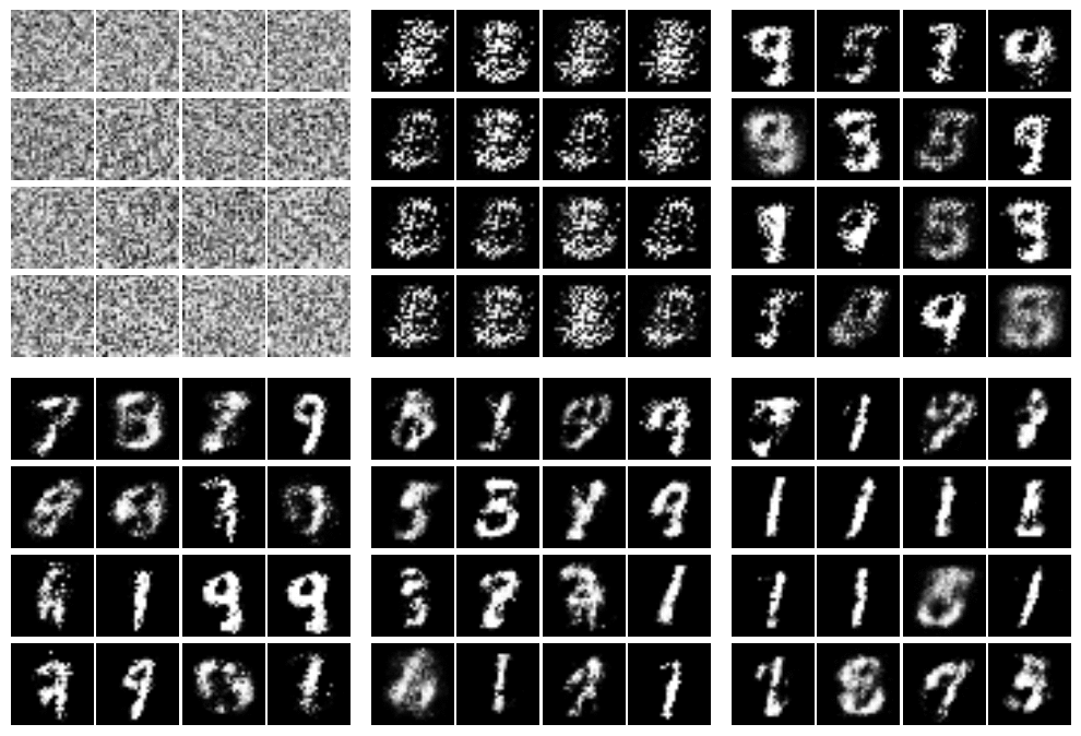
And we’re done! We can see the training process by sampling

We start with random noise and as the training goes on,
Alternative Loss Formulation
We could formulate the loss function D_loss and G_loss using different notion.
Let’s follow our intuition. This is inspired by the post about image completion in Brandon Amos’ blog.
If we think about it, the discriminator(X) wants to make all of the outputs to be 1, as per definition, we want to maximize the probability of real data. The discriminator(G_sample) wants to make all of the outputs to be 0, as again by definition,
What about generator(Z)? It wants to maximize the probability of fake data! It’s the opposite objective of
Hence, we could formulate the loss as follow.
# Alternative losses:# -------------------D_loss_real = tf.reduce_mean(tf.nn.sigmoid_cross_entropy_with_logits(D_logit_real, tf.ones_like(D_logit_real)))D_loss_fake = tf.reduce_mean(tf.nn.sigmoid_cross_entropy_with_logits(D_logit_fake, tf.zeros_like(D_logit_fake)))D_loss = D_loss_real + D_loss_fakeG_loss = tf.reduce_mean(tf.nn.sigmoid_cross_entropy_with_logits(D_logit_fake, tf.ones_like(D_logit_fake)))We’re using the Logistic Loss, following the notion above. Changing the loss functions won’t affect the GAN we’re training as this is just a different way to think and formulate the problem.
Conclusion
In this post, we looked at Generative Adversarial Network (GAN), which was published by Ian Goodfellow, et al. at NIPS 2014. We looked at the formulation of Adversarial Process and the intuition behind it.
Next, we implemented the GAN with two layer neural net for both the Generator and Discriminator Net. We then follow the algorithm presented in Goodfellow, et al, 2014 to train the GAN.
Lastly, we thought about the different way to think about GAN loss functions. In the alternative loss functions, we think intuitively about the two networks and used Logistic Loss to model the alternative loss functions.
For the full code, head to https://github.com/wiseodd/generative-models!