KL Divergence: Forward vs Reverse?

Kullback-Leibler Divergence, or KL Divergence is a measure on how “off” two probability distributions and are. It measures the distance between two probability distributions.

For example, if we have two gaussians, and , how different are those two gaussians?

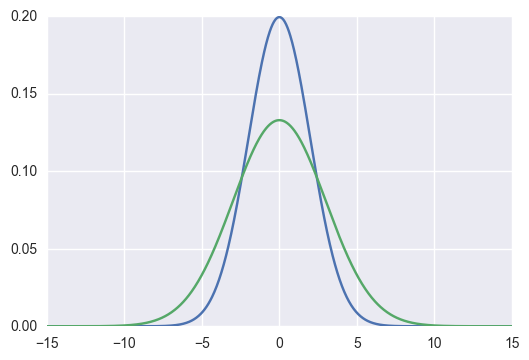
The KL Divergence could be computed as follows:

that is, for all random variable , KL Divergence calculates the weighted average on the difference between those distributions at .

KL Divergence in optimization

In optimization setting, we assume that as the true distribution we want to approximate and as the approximate distribution.

Just like any other distance functions (e.g. euclidean distance), we can use KL Divergence as a loss function in an optimization setting, especially in a probabilistic setting. For example, in Variational Bayes, we are trying to fit an approximate to the true posterior, and the process to make sure that fits is to minimize the KL Divergence between them.

However, we have to note this important property about KL Divergence: it is not symmetric. Formally, .

is called forward KL, whereas is called reverse KL.

Forward KL

In forward KL, the difference between and is weighted by . Now let’s ponder on that statement for a while.

Consider for a particular . What does that mean? As is the weight, then it doesn’t really matter what’s the value of the other term. In other words, if , there is no consequence at all to have very big difference between and . In this case, the total KL Divergence will not be affected when , as the minimum value for KL Divergence is (no distance at all, i.e. exact match). During the optimization process then, whenever , would be ignored.

Reversely, if , then the term will contribute to the overall KL Divergence. This is not good if our objective is to minimize KL Divergence. Hence, during the optimization, the difference between and will be minimized if .

Let’s see some visual examples.

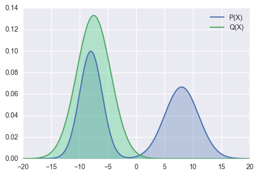
In the example above, the right hand side mode is not covered by , but it is obviously the case that ! The consequence for this scenario is that the KL Divergence would be big. The optimization algorithm then would force to take different form:

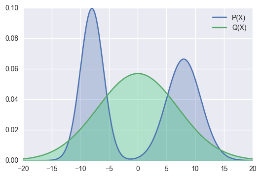
In the above example, is now more spread out, covering all . Now, there is no that are not covered by .

Although there are still some area that are wrongly covered by , this is the desired optimization result as in this form of , the KL Divergence is low.

Those are the reason why, Forward KL is known as zero avoiding, as it is avoiding whenever .

Reverse KL

In Reverse KL, as we switch the two distributions’ position in the equation, now is the weight. Still keeping that is the approximate and is the true distribution, let’s ponder some scenarios.

First, what happen if for some , in term of the optimization process? In this case, there is no penalty when we ignore .

Second, what happen if ? Now the difference between and must be as low as possible, as it now contribute to the overall divergence.

Therefore, the failure case example above for Forward KL, is the desireable outcome for Reverse KL. That is, for Reverse KL, it is better to fit just some portion of , as long as that approximate is good.

Consequently, Reverse KL will try avoid spreading the approximate. Now, there would be some portion of that will not be approximated by , i.e. .

As those properties suggest, this form of KL Divergence is know as zero forcing, as it forces to be on some areas, even if .

Conclusion

So, what’s the best KL?

As always, the answer is “it depends”. As we have seen above, both has its own characteristic. So, depending on what we want to do, we choose which KL Divergence mode that’s suitable for our problem.

In Bayesian Inference, esp. in Variational Bayes, Reverse KL is widely used. As we could see at the derivation of Variational Autoencoder, VAE also uses Reverse KL (as the idea is rooted in Variational Bayes!).

References

1. Blei, David M. “Variational Inference.” Lecture from Princeton, https://www. cs. princeton. edu/courses/archive/fall11/cos597C/lectures/variational-inference-i. pdf (2011).
2. Fox, Charles W., and Stephen J. Roberts. “A tutorial on variational Bayesian inference.” Artificial intelligence review 38.2 (2012): 85-95.