CoGAN: Learning joint distribution with GAN

The full code is available here: https://github.com/wiseodd/generative-models.

Vanilla GAN is a method to learn marginal distribution of data . Since then, it has been extended to make it learns conditional distribution . Naturally, the next extension of GAN is to learn joint distribution of data , where and are from different domain, e.g. color image and its corresponding B&W version.

Coupled GAN (CoGAN) is a method that extends GAN so that it could learn joint distribution, by only needing samples from the marginals. What it means is that we do not need to sample from joint distribution , i.e. a tuple of , during training. We only need and , samples from the marginal distributions. This property makes CoGAN very useful as collecting representing samples of joint distribution is costly due to curse of dimensionality.

Learning joint distribution by sharing weights

So, how exactly does CoGAN learn joint distribution by only using the marginals?

The trick here is to add a constraint such that high level representations of data are shared. Specifically, we constraint our networks to have the same weights on several layers. The intuition is that by constraining the weights to be identical to each other, CoGAN will converge to the optimum solution where those weights represent shared representation (joint representation) of both domains of data.

But which layers should be constrained? To answer this, we need to observe that neural nets that are used for classification tasks learn data representation in bottom-up fashion, i.e. from low level representation to high level representation. We notice that low level representation is highly specialized on data, which is not general enough. Hence, we constraint our neural net on several layers that encode the high level representation.

Intuitively, the lower level layers capture image specific features, e.g. the thickness of edges, the saturation of colors, etc. But, higher level layers capture more general features, such as the abstract representation of “bird”, “dog”, etc., ignoring the color or the thickness of the images. So, naturally, to capture joint representation of data, we want to use higher level layers, then use lower level layers to encode those abstract representation into image specific features, so that we get the correct (in general sense) and plausible (in detailed sense) images.

Using that reasoning, we then could choose which layers should be constrained. For discriminator, it should be the last layers. For generator, it should be the first layers, as generator in GAN solves inverse problem: from latent representation to image .

CoGAN algorithm

If we want to learn joint distribution of domains, then we need to use neural nets, as for each domain we need a discriminator and a generator. Fortunately, as CoGAN is centered on weight sharing, this could prove helpful to reduce the computation cost.

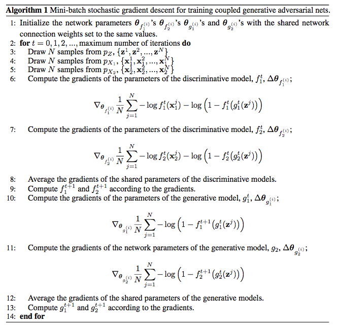
The algorithm for CoGAN for 2 domains is as follows:

Notice that CoGAN draws samples from each marginal distribution. That means, we only need 2 sets of training data. We do not need to construct specialized training data that captures joint distribution of those two domains. However, as we learn joint distribution by weight sharing on high level features, to make CoGAN training successful, we have to make sure that those two domains of data share some high level representations.

Pytorch implementation of CoGAN

In this implementation, we are going to learn joint distribution of two domains of MNIST data: normal MNIST data and rotated MNIST data (90 degree). Notice that those domains of data share the same high level representation (digit), and only differ on the presentation (low level features). Here’s the code to generate those training sets:

X_train = mnist.train.images
half = int(X_train.shape[0] / 2)

# Real image
X_train1 = X_train[:half]

# Rotated image
X_train2 = X_train[half:].reshape(-1, 28, 28)
X_train2 = scipy.ndimage.interpolation.rotate(X_train2, 90, axes=(1, 2))
X_train2 = X_train2.reshape(-1, 28*28)

Let’s declare the generators first, which are two layers fully connected nets, with first weight (input to hidden) shared:

""" Shared Generator weights """
G_shared = torch.nn.Sequential(
    torch.nn.Linear(z_dim, h_dim),
    torch.nn.ReLU(),
)

""" Generator 1 """
G1_ = torch.nn.Sequential(
    torch.nn.Linear(h_dim, X_dim),
    torch.nn.Sigmoid()
)

""" Generator 2 """
G2_ = torch.nn.Sequential(
    torch.nn.Linear(h_dim, X_dim),
    torch.nn.Sigmoid()
)

Then we make a wrapper for those nets:

def G1(z):
    h = G_shared(z)
    X = G1_(h)
    return X

def G2(z):
    h = G_shared(z)
    X = G2_(h)
    return X

Notice that G_shared are being used in those two nets.

The discriminators are also two layers nets, similar to the generators, but share weights on the last section: hidden to output.

""" Shared Discriminator weights """
D_shared = torch.nn.Sequential(
    torch.nn.Linear(h_dim, 1),
    torch.nn.Sigmoid()
)

""" Discriminator 1 """
D1_ = torch.nn.Sequential(
    torch.nn.Linear(X_dim, h_dim),
    torch.nn.ReLU()
)

""" Discriminator 2 """
D2_ = torch.nn.Sequential(
    torch.nn.Linear(X_dim, h_dim),
    torch.nn.ReLU()
)

def D1(X):
    h = D1_(X)
    y = D_shared(h)
    return y

def D2(X):
    h = D2_(X)
    y = D_shared(h)
    return y

Next, we construct the optimizer:

D_params = (list(D1.parameters()) + list(D2.parameters()) + list(D_shared.parameters()))
G_params = (list(G1.parameters()) + list(G2.parameters()) + list(G_shared.parameters()))

G_solver = optim.Adam(G_params, lr=lr)
D_solver = optim.Adam(D_params, lr=lr)

Now we are ready to train CoGAN. At each training iteration, we do these steps below. First, we sample images from both marginal training sets, and from our prior:

X1 = sample_x(X_train1, mb_size)
X2 = sample_x(X_train2, mb_size)
z = Variable(torch.randn(mb_size, z_dim))

Then, train the discriminators by using using X1 for D1 and X2 for D2. On both discriminators, we use the same z. The loss function is just vanilla GAN loss.

G1_sample = G1(z)
D1_real = D1(X1)
D1_fake = D1(G1_sample)

D1_loss = torch.mean(-torch.log(D1_real + 1e-8) - torch.log(1. - D1_fake + 1e-8))
D2_loss = torch.mean(-torch.log(D2_real + 1e-8) - torch.log(1. - D2_fake + 1e-8))

Then we just add up those loss. During backpropagation, D_shared will naturally get gradients from both D1 and D2, i.e. sum of both branches. All we need to do to get the average is to scale them:

D_loss = D1_loss + D2_loss
D_loss.backward()

# Average the gradients
for p in D_shared.parameters():
    p.grad.data = 0.5 * p.grad.data

As we have all the gradients, we could update the weights:

D_solver.step()
reset_grad()

For generators training, the procedure is similar to discriminators training, where we need to average the loss of G1 and G2 w.r.t. G_shared.

# Generator
G1_sample = G1(z)
D1_fake = D1(G1_sample)

G2_sample = G2(z)
D2_fake = D2(G2_sample)

G1_loss = torch.mean(-torch.log(D1_fake + 1e-8))
G2_loss = torch.mean(-torch.log(D2_fake + 1e-8))
G_loss = G1_loss + G2_loss

G_loss.backward()

# Average the gradients
for p in G_shared.parameters():
    p.grad.data = 0.5 * p.grad.data

G_solver.step()
reset_grad()

Results

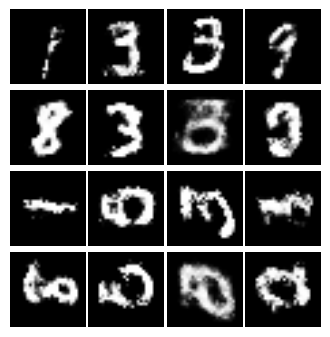
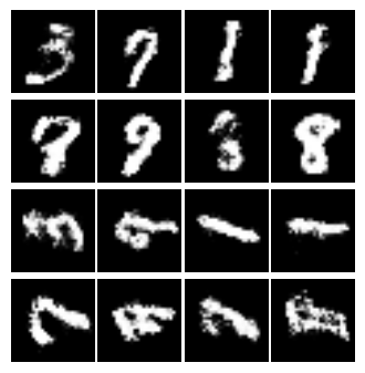
After many thousands of iterations, G1 and G2 will produce these kind of samples. Note, first two rows are the normal MNIST images, the next two rows are the rotated images. Also, the that were fed into G1 and G2 are the same so that we could see given the same latent code , we could sample that are corresponding to each other from the joint distribution.

Obviously, if we swap our nets with more powerful ones, we could get higher quality samples.

If we squint, we could see that roughly, images at the third row are the 90 degree rotation of the first row. Also, the fourth row are the corresponding images of the second row.

This is a marvelous results considering we did not explicitly show CoGAN the samples from joint distribution (i.e. a tuple of ). We only show samples from disjoint marginals. In summary, CoGAN is able to infer the joint distribution by itself.

Conclusion

In this post, we looked at CoGAN: Coupled GAN, a GAN model that is used to learn joint distribution of data from different domains.

We learned that CoGAN learned joint distribution by enforcing weight sharing constraint on its high level representation weights. We also noticed that CoGAN only needs to see samples from marginal distributions, not the joint itself.

Finally, by inspecting the samples acquired from generators, we saw that CoGAN correctly learns joint distribution, as those samples are correspond to each other.

References

1. Liu, Ming-Yu, and Oncel Tuzel. “Coupled generative adversarial networks.” Advances in Neural Information Processing Systems. 2016.