Convnet: Implementing Maxpool Layer with Numpy

Traditionally, convnet consists of several layers: convolution, pooling, fully connected, and softmax. Although it’s not true anymore with the recent development. A lot of things going on out there and the architecture of convent has been steadily (r)evolving, something like Google’s Inception module found in GoogLeNet and the recent ImageNet champion: ResNet.

Nevertheless, conv and pool layers are still the essential foundations of convnet. We’ve covered the conv layer in the last post. Now let’s dig into pool layer, especially maxpool layer.

Pool layer

Whereas conv layer applies filter to the input images, pool layer reduce the dimensionality of the output. Reducing the dimensionality of the images is a necessity in convnet as we’re dealing with a high dimensional data and a lot of filters, which implies that we will have huge amount of parameters in our convnet.

What pool layer does is simple: at each patch of the image, do a summarization operation on it. If we recall, that’s mildly similar to what conv layer does. Whereas at each location we’re taking the dot product in conv layer, we’re going to do simple summarization in a particular image patch.

The summarization operation could be any summary statistics: average, max, min, median, you name it. But, the most widely used operation is the max operation. This, combined with the adjustment of the size, padding, and stride of our image patch will result in some nice properties that are useful for our model.

Those are, mainly, the reduction of the dimensionality = less parameter = less computation burden; and slightly more robust model, because we’re taking “high level views” of our images, the network will be slightly invariant towards small changes like rotation, translation, etc.

For more about theoritical and best practices about pool layer, head to CS231n lecture page: http://cs231n.github.io/convolutional-networks/#pool.

Maxpool layer

Knowing what pool layer does, it’s trivial to think about the summarization operation. For maxpool layer, it’s just taking the maximum value of each image patch.

It’s just the same as conv layer with one exception: max instead of dot product.

Maxpool forward

As we already know that maxpool layer is similar to conv layer, implementing it is somewhat easier.

# Let say our input X is 5x10x28x28
# Our pooling parameter are: size = 2x2, stride = 2, padding = 0
# i.e. result of 10 filters of 3x3 applied to 5 imgs of 28x28 with stride = 1 and padding = 1
# First, reshape it to 50x1x28x28 to make im2col arranges it fully in column
X_reshaped = X.reshape(n \* d, 1, h, w)

# The result will be 4x9800
# Note if we apply im2col to our 5x10x28x28 input, the result won't be as nice: 40x980
X_col = im2col_indices(X_reshaped, size, size, padding=0, stride=stride)

# Next, at each possible patch location, i.e. at each column, we're taking the max index
max_idx = np.argmax(X_col, axis=0)

# Finally, we get all the max value at each column
# The result will be 1x9800
out = X_col[max_idx, range(max_idx.size)]

# Reshape to the output size: 14x14x5x10
out = out.reshape(h_out, w_out, n, d)

# Transpose to get 5x10x14x14 output
out = out.transpose(2, 3, 0, 1)

That’s it for the forward computation of maxpool layer. However, instead of getting the maximum value directly, we did an intermediate step: getting the maximum index first. This is because the index are useful for the backward computation.

At above example, we could see how maxpool layer will reduce the computation for the subsequent step. Doing 2x2 pooling with stride of 2 and no padding will essentially reduce the image dimension by half.

For example, we have this single MNIST data of 28x28:

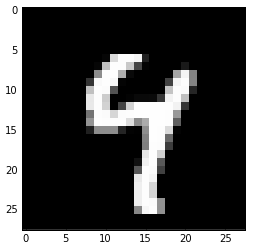
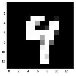
After we fed the image to our maxpool layer, the result will look like this:

Maxpool backward

Recall, how do we compute the gradient for ReLU layer. We let the gradient pass through when the ReLU result is non zero, and otherwise we block the gradient by setting it to zero.

Maxpool layer is similar, because that’s essentially what max operation do in backpropagation.

# X_col and max_idx are the intermediate variables from the forward propagation step
# Suppose our output from forward propagation step is 5x10x14x14
# We want to upscale that back to 5x10x28x28, as in the forward step
# 4x9800, as in the forward step
dX_col = np.zeros_like(X_col)

# 5x10x14x14 => 14x14x5x10, then flattened to 1x9800
# Transpose step is necessary to get the correct arrangement
dout_flat = dout.transpose(2, 3, 0, 1).ravel()

# Fill the maximum index of each column with the gradient
# Essentially putting each of the 9800 grads
# to one of the 4 row in 9800 locations, one at each column
dX_col[max_idx, range(max_idx.size)] = dout_flat

# We now have the stretched matrix of 4x9800, then undo it with col2im operation
# dX would be 50x1x28x28
dX = col2im_indices(dX_col, (n \* d, 1, h, w), size, size, padding=0, stride=stride)

# Reshape back to match the input dimension: 5x10x28x28
dX = dX.reshape(X.shape)

Recall the ReLU gradient is dX[X <= 0] = 0, as we’re doing max(0, x) in ReLU. We’re basically applying that to our stretched image patches. Only, we start with 0 matrix and put the gradient in the correct location, and we’re taking the max of the image patch, instead of comparing it with 0 like we do in ReLU.

Conclusion

We see that pool layer, specifically maxpool layer is similar to conv and ReLU layer. It’s similar as conv as we need to stretch our input image with im2col to get the all possible image patches where we are going to take the maximum value over. It’s similar as ReLU as we’re doing the same operation: max.

We also see that doing maxpool with certain parameters, e.g. 2x2 maxpool with stride of 2 and padding of 0 will essentially halve the dimension of the input.