Implementing BatchNorm in Neural Net

BatchNorm a.k.a Batch Normalization is a relatively new technique proposed by Ioffe & Szegedy in 2015. It promises us acceleration in training (deep) neural net.

One difficult thing about training a neural net is to choose the initial weights. BatchNorm promises the remedy: it makes the network less dependant to the initialization strategy. Another key points are that it enables us to use higher learning rate. They even go further to state that BatchNorm could reduce the dependency on Dropout.

BatchNorm: the algorithm

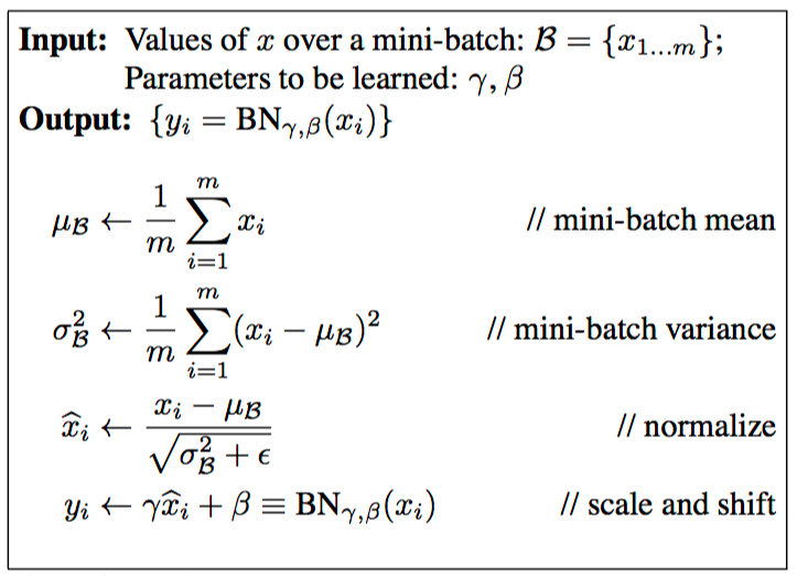
The main idea of BatchNorm is this: for the current minibatch while training, in each hidden layer, we normalize the activations so that its distribution is Standard Normal (zero mean and one standard deviation). Then, we apply a linear transform to it with learned parameters so that the network could learn what kind of distribution is the best for the layer’s activations.

This in turn will make the gradient flows better as activations saturation is not a problem anymore. Recall that activations saturation kills neurons in case of ReLU and makes gradient vanish or explode in case of sigmoid.

It enables us to be less careful with weights initialization as we don’t need to worry anymore if our weights initialization makes the activations saturated too quickly which in turn make the gradient explode. BatchNorm takes care of that.

The forward propagation of BatchNorm is shown below:

Pretty simple right? We just need to compute the activations mean and variance over the current minibatch and normalize the activations with that. What could go wrong.

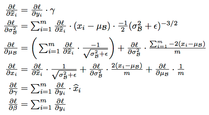
Well, we’re training neural net with Backpropagation here, so that algorithm is half the story. We still need to derive the backprop scheme for the BatchNorm layer. Which is given by this:

If the above derivation doesn’t make any sense, you could try reading this in combination with computational graph approach of backprop in CS231 lecture.

Now that we know how to do forward and backward propagation for BatchNorm, let’s try to implement that.

Training with BatchNorm

As always, I will reuse the code from previous posts. It’s in my repo here: https://github.com/wiseodd/hipsternet.

def batchnorm_forward(X, gamma, beta):
    mu = np.mean(X, axis=0)
    var = np.var(X, axis=0)

    X_norm = (X - mu) / np.sqrt(var + 1e-8)
    out = gamma * X_norm + beta

    cache = (X, X_norm, mu, var, gamma, beta)

    return out, cache, mu, var

This is the forward propagation algorithm. It’s simple. However, remember that we’re normalizing each dimension of activations. So, if our activations over a minibatch is MxN matrix, then we want the mean and variance to be 1xN: one value of mean and variance for each dimension. So, if we normalize our activations matrix with that, each dimension will have zero mean and one variance.

At the end, we’re also spitting out the intermediate variable used for normalization as they’re essential for the backprop.

This is how we use that above method:

# Input to hidden
h1 = X @ W1 + b1

# BatchNorm
h1, bn1_cache, mu, var = batchnorm_forward(h1, gamma1, beta1)

# ReLU
h1[h1 < 0] = 0

In the BatchNorm paper, they insert the BatchNorm layer before nonlinearity. But it’s not set in a stone.

For the backprop, here’s the implementation:

def batchnorm_backward(dout, cache):
    X, X_norm, mu, var, gamma, beta = cache

    N, D = X.shape

    X_mu = X - mu
    std_inv = 1. / np.sqrt(var + 1e-8)

    dX_norm = dout * gamma
    dvar = np.sum(dX_norm * X_mu, axis=0) * -.5 * std_inv**3
    dmu = np.sum(dX_norm * -std_inv, axis=0) + dvar * np.mean(-2. * X_mu, axis=0)

    dX = (dX_norm * std_inv) + (dvar * 2 * X_mu / N) + (dmu / N)
    dgamma = np.sum(dout * X_norm, axis=0)
    dbeta = np.sum(dout, axis=0)

    return dX, dgamma, dbeta

For the explanation of the code, refer to the derivation of the BatchNorm gradient in the last section. As we can see, we’re also returning derivative of gamma and beta: the linear transform for BatchNorm. It will be used to update the model, so that the net could also learn them.

# h1
dh1 = dh2 @ W2.T

# ReLU
dh1[h1 <= 0] = 0

# Dropout h1
dh1 *= u1

# BatchNorm
dh1, dgamma1, dbeta1 = batchnorm_backward(dh2, bn2_cache)

Remember, the order of backprop is important! We will get wrong result if we swap the BatchNorm gradient with ReLU gradient for example.

Inference with BatchNorm

One more thing we need to take care of is that we want to fix the normalization at test time. That means we don’t want to normalize our activations with the test set. Hence, as we’re essentially using SGD, which is stochastic, we’re going to estimate the mean and variance of our activations using running average.

# BatchNorm training forward propagation
h2, bn2*cache, mu, var = batchnorm_forward(h2, gamma2, beta2)
bn_params['bn2_mean'] = .9 * bn*params['bn2_mean'] + .1 * mu
bn_params['bn2_var'] = .9 * bn*params['bn2_var'] + .1 * var

There, we store each BatchNorm layer’s running mean and variance while training. It’s a decaying running average.

Then, at the test time, we just use that running average for the normalization:

# BatchNorm inference forward propagation
h2 = (h2 - bn_params['bn2_mean']) / np.sqrt(bn_params['bn2_var'] + 1e-8)
h2 = gamma2 \* h2 + beta2

And that’s it. Our implementation of BatchNorm is now complete. Now the test!

Test and Comparison

We’re going to use a three layer network with 256 neurons in each hidden layer and minibatch size of 256. We use 1000 iterations of Adam for the optimization. We’re also using Dropout with probability of 0.5.

First, let’s test the claim of BatchNorm makes the network less dependant on weights initialization. We’re going to just use this initialization scheme: W1=np.random.randn(D, H).

# learning rate = 1e-2

# With BatchNorm:
Iter-100 loss: 14.755845933600622
Iter-200 loss: 6.411304732436082
Iter-300 loss: 3.8945102118430466
Iter-400 loss: 2.4634817943096805
Iter-500 loss: 1.660556228305082
Iter-600 loss: 1.279642232187109
Iter-700 loss: 1.0457504142354406
Iter-800 loss: 0.9400718897268598
Iter-900 loss: 1.0161870928408856
Iter-1000 loss: 0.833607292631844

adam => mean accuracy: 0.8853, std: 0.0079

# Without BatchNorm:
Iter-100 loss: 49.73374055679555
Iter-200 loss: 46.61991288615765
Iter-300 loss: 44.1475586165201
Iter-400 loss: 42.57901406076491
Iter-500 loss: 41.30118729832132
Iter-600 loss: 38.58016074343413
Iter-700 loss: 36.495641945628186
Iter-800 loss: 34.454519834002745
Iter-900 loss: 32.40071379522495
Iter-1000 loss: 30.35279106760543

adam => mean accuracy: 0.1388, std: 0.0219

It works wonder! The “unproper” initialization seems to make the non-BatchNorm network’s gradients vanish, so it can’t learn well. With BatchNorm, the optimization just zip through and converging in much faster speed.

Let’s do one more test. This time we’re using the proper initialization: Xavier / 2. How is BatchNorm compared to Dropout? In the paper, the authors made a point that by using BatchNorm, the network could be less dependant to Dropout.

# With only BatchNorm
rmsprop => mean accuracy: 0.9740, std: 0.0016

# With only Dropout
rmsprop => mean accuracy: 0.9692, std: 0.0006

# With nothing
rmsprop => mean accuracy: 0.9640, std: 0.0071

The network with BatchNorm performs much better!

However, not all are rosy. Remember the no free lunch theorem. BatchNorm has a drawback: it makes our training slower. Here’s the comparison:

# With BatchNorm:
python run.py  81.12s user 7.34s system 184% cpu 47.958 total

# Without BatchNorm:
python run.py  63.94s user 4.42s system 186% cpu 36.616 total

With BatchNorm, we’re expecting 30% slow down.

Conclusion

In this post, we’re looking at the relatively new technique for training neural nets, called BatchNorm. It does just that: normalizing the activations of the network at each minibatch, so that the activations will be approximately Standard Normal distributed.

We also implemented BatchNorm in three layers network, then tested it using various parameters. It’s by no mean rigorous, but we could catch a glimpse of BatchNorm in action.

In the test, we found that by using BatchNorm, our network become more tolerant to bad initialization. BatchNorm network also outperform Dropout in our test setting. However, those are with the expense of 30% increase of training time.