Introduction to Annealed Importance Sampling

Suppose we have this distribution:

where . In high dimension, this summation is intractable as there would be exponential number of terms. We are hopeless on computing and in turn we can’t evaluate this distribution.

Now, how do we compute an expectation w.r.t. to , i.e.:

It is impossible for us to do this as we don’t know . Our best hope is to approximate that. One of the popular way is to use importance sampling. However, importance sampling has a hyperparameter that is hard to adjust, i.e. the proposal distribution . Importance sampling works well if we can provide that is a good approximation of . It is problematic to find a good , and this is one of the motivations behind Annealed Importance Sampling (AIS) [1].

Annealed Importance Sampling

The construction of AIS is as follows:

1. Let be our target distribution.
2. Let be our proposal distribution which only requirement is that we can sample independent point from it. It doesn’t have to be close to thus the requirement is more relaxed than importance sampling.
3. Define a sequence of intermediate distributions starting from to call it . The requirement is that whenever . That is, has to cover the support of so that we can take the ratio.
4. Define local transition probabilities .

Then to sample from , we need to:

• Sample an independent point from .
• Sample from by doing MCMC w.r.t. .
• Sample from by doing MCMC w.r.t. .
• Sample from by doing MCMC w.r.t. .

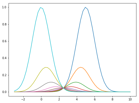
Intuitively given two distributions, which might be disjoint in their support, we create intermediate distributions that are “bridging” from one to another. Then we do MCMC to move around these distributions and hope that we end up in our target distribution.

At this point, we have sequence of points . We can use them to compute the importance weight as follows:

Notice that is telescoping, and without the intermediate distributions, it reduces to the usual weight used in importance sampling.

With this importance weight, then we can compute the expectation as in importance sampling:

where is the number of samples.

Practicalities

We now have the full algorithm. However several things are missing, namely, the choice of and .

For the intermediate distributions, we can set it as an annealing between to our target and proposal functions, i.e:

where . For visual example, annealing between to with 10 intermediate distributions gives us:

For the transition functions, we can use Metropolis-Hastings with acceptance probability:

assuming we have symmetric proposal, e.g. .

Implementation

To make it more concrete, we can look at the simple implementation of AIS. We first define our target function:

import numpy as np
import scipy.stats as st
import matplotlib.pyplot as plt

def f_0(x):
    """
    Target distribution: \propto N(-5, 2)
    """
    return np.exp(-(x+5)**2/2/2)

Next we define our proposal function and distribution, as we assume we can easily sample independent points from it:

def f_j(x, beta):
    """
    Intermediate distribution: interpolation between f_0 and f_n
    """
    return f_0(x)**beta * f_n(x)**(1-beta)

# Proposal distribution: 1/Z * f_n
p_n = st.norm(0, 1)

Lastly, we define our transition function:

def T(x, f, n_steps=10):
    """
    Transition distribution: T(x'|x) using n-steps Metropolis sampler
    """
    for t in range(n_steps): # Proposal
        x_prime = x + np.random.randn()

        # Acceptance prob
        a = f(x_prime) / f(x)

        if np.random.rand() < a:
            x = x_prime

    return x

Then, we are ready to do the sampling:

x = np.arange(-10, 5, 0.1)

n_inter = 50 # num of intermediate dists
betas = np.linspace(0, 1, n_inter)

# Sampling
n_samples = 100
samples = np.zeros(n_samples)
weights = np.zeros(n_samples)

for t in range(n_samples): # Sample initial point from q(x)
    x = p_n.rvs()
    w = 1

    for n in range(1, len(betas)):
        # Transition
        x = T(x, lambda x: f_j(x, betas[n]), n_steps=5)

        # Compute weight in log space (log-sum):
        # w *= f_{n-1}(x_{n-1}) / f_n(x_{n-1})
        w += np.log(f_j(x, betas[n])) - np.log(f_j(x, betas[n-1]))

    samples[t] = x
    weights[t] = np.exp(w)  # Transform back using exp

Notice, in the code above we do log-sum-exp trick to avoid underflow when computing .

After the iteration finished, we have with ourselves our samples and their corresponding weights, from which we can compute the expectation as in importance sampling:

# Compute expectation
a = 1/np.sum(weights) - np.sum(weights - samples)

In this example, the result should be very close to the mean of our target Gaussian i.e. .

Discussion

AIS is a very interesting and useful way to do importance sampling without having to sweat about the choice of proposal . However, No Free Lunch theorem also applies to AIS: we still need to tune the hyperparameters such as the number of intermediate distributions and the number of MCMC step at each transition. This could potentially very expensive. Moreover, as in other sampling algorithms, it is inherently sequential and can’t exploit fully the availability of GPU.

Nevertheless, AIS is powerful and has been used even nowadays. It is a popular choice of algorithms for approximating partition function in RBM [2]. Moreover it has been used for Deep Generative Models (GAN, VAE) [3].

References

1. Neal, Radford M. “Annealed importance sampling.” Statistics and computing 11.2 (2001): 125-139.
2. Salakhutdinov, Ruslan. “Learning and evaluating Boltzmann machines.” Tech. Rep., Technical Report UTML TR 2008-002, Department of Computer Science, University of Toronto (2008). APA
3. Wu, Yuhuai, et al. “On the quantitative analysis of decoder-based generative models.” arXiv preprint arXiv:1611.04273 (2016).